In the previous section, we dealt with the multiplication system and defined the infinite and finite multiplication factors. This section was about conditions for a stable, self-sustained fission chain reaction and maintaining such conditions. This problem contains no information about the spatial distribution of neutrons because it is a point geometry problem. We have characterized the effects of the global distribution of neutrons simply by a non-leakage probability (thermal or fast), which, as stated earlier, increases toward a value of one as the reactor core becomes larger.
To design a nuclear reactor properly, predicting how the neutrons will be distributed throughout the system is highly important. This is a very difficult problem because the neutrons interact differently with different environments (moderator, fuel, etc.) in a reactor core. Neutrons undergo various interactions when they migrate through the multiplying system. To a first approximation, the overall effect of these interactions is that the neutrons undergo a kind of diffusion in the reactor core, much like the diffusion of one gas in another. This approximation is usually known as the diffusion approximation, based on the neutron diffusion theory. This approximation allows solving such problems using the diffusion equation.
In this chapter, we will introduce the neutron diffusion theory. We will examine the spatial migration of neutrons to understand the relationships between reactor size, shape, and criticality and determine the spatial flux distributions within power reactors. The diffusion theory provides a theoretical basis for neutron-physical computing of nuclear cores. It must be added many neutron-physical codes are based on this theory.
First, we will analyze the spatial distributions of neutrons, and we will consider a one-group diffusion theory (mono-energetic neutrons) for a uniform non-multiplying medium. That means that the neutron flux and cross-sections have already been averaged over energy. Such a relatively simple model has the great advantage of illustrating many important features of the spatial distribution of neutrons without the complexity introduced by the treatment of effects associated with the neutron energy spectrum.
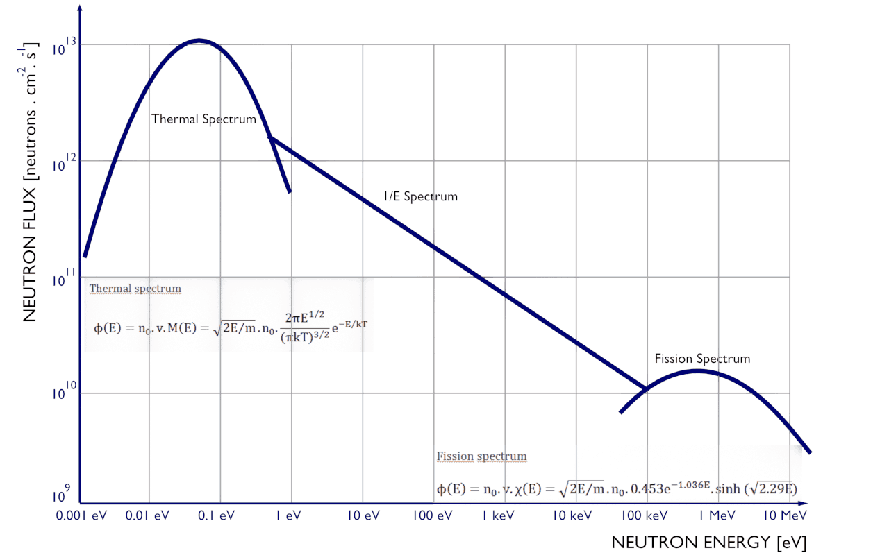
See also: Neutron Flux Spectra.
Moreover, mathematical methods used to analyze a one-group diffusion equation are the same as those applied in more sophisticated and accurate methods such as multi-group diffusion theory. Subsequently, the one-group diffusion theory will be applied in simple geometries on a uniform multiplying medium (a homogeneous “nuclear reactor”). Finally, the multi-group diffusion theory will be applied in simple geometries on a non-uniform multiplying medium (a heterogenous “nuclear reactor”).
Transport theory is relatively simple in principle, and an exact transport equation governing this phenomenon can easily be derived. This equation is called the Boltzmann transport equation, and the entire study of transport theory focuses on the study of this equation. In general, the neutron balance can be expressed graphically as:
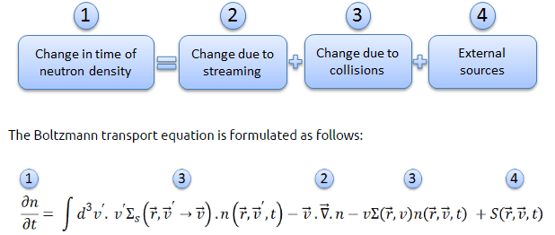
Boltzmann Transport Equation

The Boltzman transport equation is a balance statement that conserves neutrons. Each term represents a gain or a loss of a neutron, and the balance, in essence, claims that neutrons gained equals neutrons lost. It must be added that it is much easier to derive the Boltzmann transport equation than to solve it. Deterministic methods solve the Boltzmann transport equation in a numerically approximated manner everywhere throughout a modeled system. This task demands enormous computational resources because the problem has many dimensions. But the Boltzmann transport equation can be treated in a rather straightforward way. This simplified version of the Boltzmann transport equation is just the neutron diffusion equation. Naturally, many assumptions must be fulfilled when using the diffusion equation, but the diffusion equation usually provides a sufficiently accurate approximation to the exact transport equation.
Nowadays, reactor core analyses and design can be performed using nodal two-group diffusion methods. These methods are based on pre-computed assembly homogenized cross-sections and assembly discontinuity factors (pin factors) obtained by single assembly calculation with reflective boundary conditions (infinite lattice). Two methods exist for the calculation of the pre-computed assembly cross-sections and pin factors.
- Deterministic methods that solve the Boltzmann transport equation.
- Stochastic methods are known as Monte Carlo methods that model the problem almost exactly.
These methods are very efficient and accurate when applied to the current Pressurized Water Reactors (PWRs) or Boiling Water Reactors (BWRs).
Derivation of One-group Diffusion Equation
The derivation of the diffusion equation depends on Fick’s law, which states that solute diffuses from high concentration to low. But first, we have to define a neutron flux and neutron current density. The neutron flux is used to characterize the neutron distribution in the reactor, and it is the main output of solutions of diffusion equations. The neutron flux, φ, does not characterize the flow of neutrons. There may be no flow of neutrons, yet many interactions may occur (I = Σ.φ). The neutrons move in random directions and hence may not flow. Therefore the neutron flux φ is more closely related to densities. Neutrons will exhibit a net flow when there are spatial differences in their density. Hence we can have a flux of neutron flux! This flux of neutron flux is called the neutron current density.
Ф = n.v
where:
Ф – neutron flux (neutrons.cm-2.s-1)
n – neutron density (neutrons.cm-3)
v – neutron velocity (cm.s-1)
The neutron flux, the number of neutrons crossing through some arbitrary cross-sectional unit area in all directions per unit time, is a scalar quantity. Therefore it is also known as the scalar flux. The expression Ф(E).dE is the total distance traveled during one second by all neutrons with energies between E and dE located in 1 cm3.
The connection to the reaction rate, respectively, the reactor power is obvious. Knowledge of the neutron flux (the total path length of all the neutrons in a cubic centimeter in a second) and the macroscopic cross-sections (the probability of having an interaction per centimeter path length) allows us to compute the rate of interactions (e.g.,, rate of fission reactions). The reaction rate (the number of interactions taking place in that cubic centimeter in one second) is then given by multiplying them together:
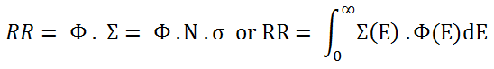
where:
Ф – neutron flux (neutrons.cm-2.s-1)
σ – microscopic cross-section (cm2)
N – atomic number density (atoms.cm-3)
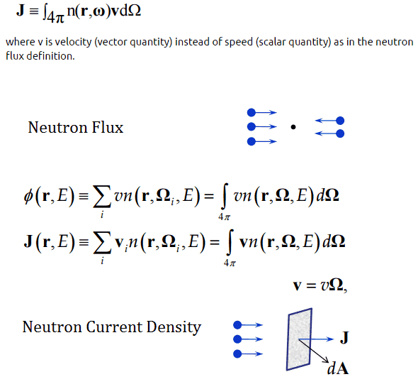
This flux of neutron flux is called the neutron current density. We have to distinguish between the neutron flux and the neutron current density. Although both physical quantities have the same units, namely, neutrons.cm-2.s-1, their physical interpretations are different. In contrast to the neutron flux, the neutron current density is the number of neutrons crossing through some arbitrary cross-sectional unit area in a single direction per unit time (a surface is perpendicular to the direction of the beam). The neutron current density is a vector quantity.
The vector J is defined as the following integral:
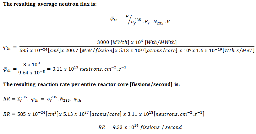
A typical thermal reactor contains about 100 tons of uranium with an average enrichment of 2% (do not confuse it with the enrichment of the fresh fuel). If the reactor power is 3000MWth, determine the reaction rate and the average core thermal flux.
Solution:
Multiplying the reaction rate per unit volume (RR = Ф . Σ) by the total volume of the core (V) gives us the total number of reactions occurring in the reactor core per unit time. But we also know the amount of energy released per one fission reaction to be about 200 MeV/fission. Now, it is possible to determine the rate of energy release (power) due to the fission reaction. It is given by the following equation:
P = Ф . Σf . Er . V = Ф . NU235 . σf235 . Er . V
where:
P – reactor power (MeV.s-1)
Ф – neutron flux (neutrons.cm-2.s-1)
σ – microscopic cross section (cm2)
N – atomic number density (atoms.cm-3)
Er – the average recoverable energy per fission (MeV / fission)
V – total volume of the core (m3)
The amount of fissile 235U per the volume of the reactor core.
m235 [g/core] = 100 [metric tons] x 0.02 [g of 235U / g of U] . 106 [g/metric ton] = 2 x 10⁶ grams of 235U per the volume of the reactor core
The atomic number density of 235U in the volume of the reactor core:
N235 . V = m235 . NA / M235
= 2 x 10⁶ [g 235 / core] x 6.022 x 10²³ [atoms/mol] / 235 [g/mol]
= 5.13 x 1027 atoms / core
The microscopic fission cross-section of 235U (for thermal neutrons):
σf235 = 585 barns
The average recoverable energy per 235U fission:
Er = 200.7 MeV/fission
Fick’s Law
In chemistry, Fick’s law states that:
Suppose the concentration of a solute in one region is greater than in another of a solution. In that case, the solute diffuses from the region of higher concentration to the region of lower concentration, with a magnitude that is proportional to the concentration gradient.
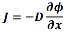
In one (spatial) dimension, the law is:
where:
- J is the diffusion flux,
- D is the diffusion coefficient,
- φ (for ideal mixtures) is the concentration.
The use of this law in nuclear reactor theory leads to the diffusion approximation.
Fick’s law in reactor theory stated that:
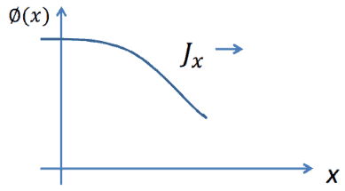
The current density vector J is proportional to the negative of the gradient of the neutron flux. The proportionality constant is called the diffusion coefficient and is denoted by the symbol D.
In one (spatial) dimension, the law is:
where:
- J is the neutron current density (neutrons.cm-2.s-1) along the x-direction, the net flow of neutrons that pass per unit of time through a unit area perpendicular to the x-direction.
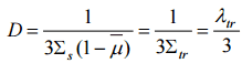
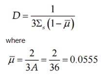
- D is the diffusion coefficient, it has the unit of cm, and it is given by:
- φ is the neutron flux, the number of neutrons crossing through some arbitrary cross-sectional unit area in all directions per unit time.

The generalized Fick’s law (in three dimension) is:
![]()
where J denotes the diffusion flux vector. Note that the gradient operator turns the neutron flux, which is a scalar quantity into the neutron current, which is a vector quantity.
Physical Interpretation
 The physical interpretation is similar to the fluxes of gases. The neutrons exhibit a net flow in the direction of least density. This is a natural consequence of greater collision densities at positions of greater neutron densities.
Consider neutrons passing through the plane at x=0 from left to right due to collisions to the plane’s left. Since the concentration of neutrons and the flux is larger for negative values of x, there are more collisions per cubic centimeter on the left. Therefore more neutrons are scattered from left to right, then the other way around. Thus the neutrons naturally diffuse toward the right.
Validity of Fick’s Law
It must be emphasized that Fick’s law is an approximation and was derived under the following conditions:
- Infinite medium. This assumption is necessary to allow integration of overall space but flux contributions are negligible beyond a few mean free paths (about three mean free paths) from boundaries of the diffusive medium.
- Sources or sinks. Derivation of Fick’s law assumes that the contribution to the flux is mostly from elastic scattering reactions. Source neutrons contribute to the flux if they are more than a few mean free paths from a source.
- Uniform medium. Derivation of Fick’s law assumes that a uniform medium was used. There are different scattering properties at the boundary (interface) between the two media.
- Isotropic scattering. Isotropic scattering occurs at low energies but is not true in general. Anisotropic scattering can be corrected by modification of the diffusion coefficient (based on transport theory).
- Low absorbing medium. Fick’s law derivation assumes (an expansion in Taylor’s series) that the neutron flux, φ, is slowly varying. Large variations in φ occur when Σa (neutron absorption) is large (compared to Σs). Σa << Σs
- Time-independent flux. Derivation of Fick’s law assumes that the neutron flux is independent of time.
To some extent, these limitations are valid in every practical reactor. Nevertheless, Fick’s law gives a reasonable approximation. For more detailed calculations, higher-order methods are available.
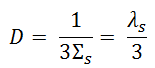
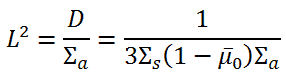
where Σs is the macroscopic scattering cross-section and λs is the scattering mean free path.
However, we can express the diffusion coefficient from the more advanced transport theory in terms of transport and absorption cross-sections:
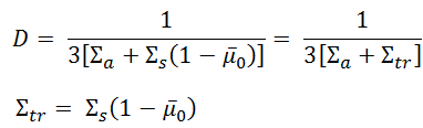
where:
- λtr is the transport mean free path
- Σa is the macroscopic absorption cross-section.
- Σtr is the macroscopic transport cross-section
- μ0 is the average value of the cosine of the angle in the lab system
In a weakly absorbing medium where Σa << Σs the diffusion coefficient can be approximately calculated as:
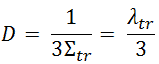
The transport means free path (λtr) is an average distance a neutron will move in its original direction after an infinite number of scattering collisions.
![]()
is the average value of the cosine of the angle in the lab system at which neutrons are scattered in the medium. It can be calculated for most of the neutron energies as (A is the mass number of target nucleus):


Operational changes that affect the diffusion length
The diffusion coefficient is a very important parameter in thermal reactors, and its magnitude can be changed during reactor operation. Since the diffusion coefficient is dependent on the macroscopic scattering cross-section, Σs, we will study the impacts of operational changes on this parameter.
Change in the moderator temperature
The diffusion coefficient, D, is sensitive, especially on the change in the moderator temperature.
In short, as the moderator temperature increases, the diffusion coefficient also slightly increases.
This increase in the diffusion coefficient is especially due (Σs=σs.NH2O) to a decrease in the macroscopic scattering cross-section, Σs=σs.NH2O, caused by the thermal expansion of water (a decrease in the atomic number density).
Calculation of Diffusion Coefficient
The scattering cross-section of carbon at 1 eV is 4.8 b (4.8×10⁻²⁴ cm2). Calculate the diffusion coefficient and the transport mean free path.
Solution:
We will calculate the diffusion according to the advanced formula:
First, we have to determine the atomic number density of carbon and then the scattering macroscopic cross-section.
Density:
MC = 12
NC = ρ . Na / MC
= (2.2 g/cm3)x(6.022×1023 nuclei/mol)/ (12 g/mol)
= 1.1×10²³ nuclei / cm3
σs12C = 4.8 b
Σs12C = 4.8×10-24 x 1.1×1023 = 0.528 cm-1
the diffusion coefficient is then:
D = 1 / (3 x 0.528 x 0.9445) = 0.668 cm
the transport mean free path
λtr = 3 x D = 2.005 cm
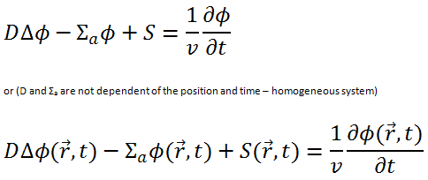
Neutron Balance – Continuity Equation
The mathematical formulation of neutron diffusion theory is based on the balance of neutrons in a differential volume element. Since neutrons do not disappear (β decay is neglected), the following neutron balance must be valid in an arbitrary volume V.
rate of change of neutron density = production rate – absorption rate – leakage rate
where
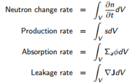
Substituting for the different terms in the balanced equation and by dropping the integral over (because the volume V is arbitrary), we obtain:
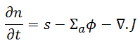
where
- n is the density of neutrons,
- s is the rate at which neutrons are emitted from sources per cm3 (either from external sources (S) or from fission (ν.Σf.Ф)),
- J is the neutron current density vector
- Ф is the scalar neutron flux
- Σa is the macroscopic absorption cross-section
In steady-state, when n is not a function of time:
![]()
The Diffusion Equation
In previous chapters, we introduced two bases for the derivation of the diffusion equation:
Fick’s law:
![]()
which states that neutrons diffuse from high concentration (high flux) to low concentration.
Continuity equation:
which states that rate of change of neutron density = production rate – absorption rate – leakage rate.
We return now to the neutron balance equation and substitute the neutron current density vector by J = -D∇Ф. Assuming that ∇.∇ = ∇2 = Δ (therefore div J = -D div (∇Ф) = -DΔФ) we obtain the diffusion equation.

The derivation of the diffusion equation is based on Fick’s law which is derived under many assumptions. Therefore, the diffusion equation cannot be exact or valid at places with strongly differing diffusion coefficients or in strongly absorbing media. This implies that the diffusion theory may show deviations from a more accurate solution of the transport equation in the proximity of external neutron sinks, sources, and media interfaces.
See also : Microscopic Cross-section
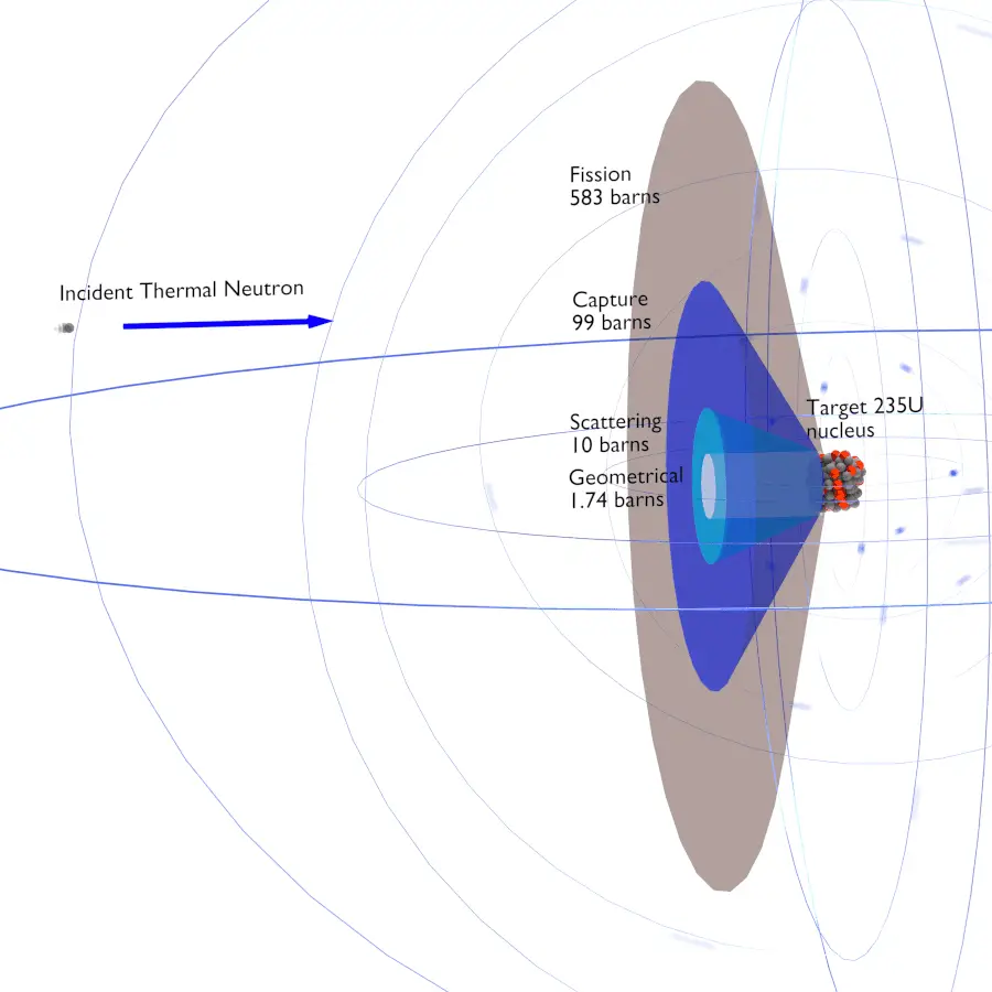
The extent to which neutrons interact with nuclei is described in terms of quantities known as cross-sections. Cross-sections are used to express the likelihood of particular interaction between an incident neutron and a target nucleus. It must be noted this likelihood does not depend on real target dimensions. In conjunction with the neutron flux, it enables the calculation of the reaction rate, for example, to derive the thermal power of a nuclear power plant. The standard unit for measuring the microscopic cross-section (σ-sigma) is the barn, equal to 10-28 m2. This unit is very small. Therefore barns (abbreviated as “b”) are commonly used.
The cross-section σ can be interpreted as the effective ‘target area’ that a nucleus interacts with an incident neutron. The larger the effective area, the greater the probability of reaction. This cross-section is usually known as the microscopic cross-section.
The concept of the microscopic cross-section is therefore introduced to represent the probability of a neutron-nucleus reaction. It can be shown that whether a neutron will interact with a certain volume of material depends not only on the microscopic cross-section of the individual nuclei but also on the density of nuclei within that volume. It depends on the N.σ factor. This factor is therefore widely defined, and it is known as the macroscopic cross-section.
The difference between the microscopic and macroscopic cross-sections is extremely important. The microscopic cross-section represents the effective target area of a single nucleus, while the macroscopic cross-section represents the effective target area of all of
the nuclei contained in a certain volume.
Boundary Conditions
To solve the diffusion equation, which is a second-order partial differential equation throughout the reactor volume, it is necessary to specify certain boundary conditions. It is very dependent on the complexity of a certain problem. One-dimensional problems solutions of diffusion equation contain two arbitrary constants. Therefore, we need two boundary conditions to determine these coefficients to solve a one-dimensional one-group diffusion equation. The most convenient boundary conditions are summarized in the following few points:
The diffusion equation is mostly solved in media with high densities, such as neutron moderators (H2O, D2O, or graphite). The problem is usually bounded by air. The mean free path of the neutron in the air is much larger than in the moderator so that it is possible to treat it as a vacuum in neutron flux distribution calculations. The vacuum boundary condition supposes that no neutrons are entering a surface.
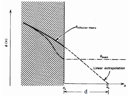
If we consider that no neutrons are reflected from the vacuum back to the volume, the following condition can be derived from Fick’s law:
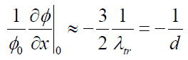
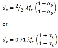
Where d ≈ ⅔ λtr is known as the extrapolated length, for homogeneous, weakly absorbing media, an exact solution of the mono-energetic transport equation in this case yields d ≈ 0.7104 λtr. The geometric interpretation of the previous equation is that the relative neutron flux near the boundary has a slope of -1/d, i.e., the flux would extrapolate linearly to 0 at a distance d beyond the boundary. This zero flux boundary condition is more straightforward and can be written mathematically as:

If d is not negligible, physical dimensions of the reactor are increased by d, and extrapolated boundary is formulated with dimension Re = R + d, and this condition can be written as Φ(R + d) = Φ(Re) = 0.
It may seem the flux goes to 0 at an extrapolated length beyond the boundary. This interpretation is not correct. The flux cannot go to zero in a vacuum because there are no absorbers to absorb the neutrons. The flux only appears to be heading to the zero value at the extrapolation point.
Note that the equation d ≈ 0.7104 λtr is applicable to plane boundaries only. The formulas for curved boundaries can differ slightly. However, the difference is small unless the radius of curvature of the boundary is of the same order of magnitude as the extrapolated length.
Typical values of the extrapolated length:
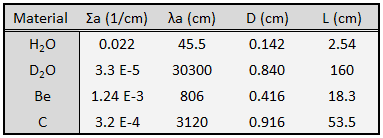
The most common moderators have following diffusion coefficients (for thermal neutrons):
D(H2O) = 0.142 cm
D(D2O) = 0.84 cm
D(Be) = 0.416 cm
D(C) = 0.916 cm
The thermal neutron extrapolated lengths are given by:
d ≈ 0.7104 λtr = 0.7104 x 3 x D
therefore:
H2O: d ≈ 0.30 cm
D2O: d ≈ 1.79 cm
Be: d ≈ 0.88 cm
C: d ≈ 1.95 cm
As can be seen, this approximation is valid when the dimension L of the diffusing medium is much larger than the extrapolated length, L >> d.
![]()
These conditions are often used to eliminate unnecessary functions from solutions.
It must be added, as J must be continuous, the flux gradient will show a jump if the diffusion coefficients in both media differ from each other.
On this special interface, we shall apply an albedo boundary condition to represent the neutron reflector. Albedo, the latin word for “whiteness”, was defined by Lambert as the fraction of the incident light reflected diffusely by a surface.
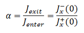
In reactor engineering, albedo, or the reflection coefficient, is defined as the ratio of exiting to entering neutrons, and we can express it in terms of neutron currents as:
For sufficiently thick reflectors, it can be derived that albedo becomes

where Drefl is the diffusion coefficient in the reflector and the Lrefl is the diffusion length in the reflector.
If we are not interested in the neutron flux distribution in the reflector (let say in the slab B) but only in the effect of the reflector on the neutron flux distribution in the medium (let say in slab A), the albedo of the reflector can be used as a boundary condition for the diffusion equation solution. This boundary condition is similar to the vacuum boundary condition, i.e., Φ(Ralbedo) = 0, where Ralbedo = R + de and
Diffusion Length of Neutron
During the diffusion equation solution, we often meet with a very important parameter that describes the behavior of neutrons in a medium.
The solution of diffusion equation (let assume the simplest diffusion equation) usually starts by division of entire equation by diffusion coefficient:
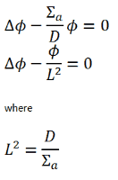
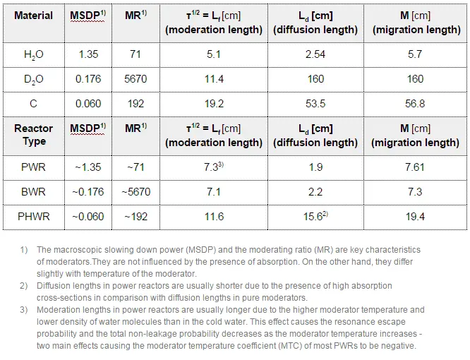
The term L2 is called the diffusion area (and L is called the diffusion length). For thermal neutrons with an energy of 0.025 eV, a few values of L are given in the table below.
Physical Meaning of the Diffusion Length
It is interesting to try to interpret the “physical” meaning of the diffusion length. The physical meaning of the diffusion length can be seen by calculating the mean square distance that a neutron travels in the one direction from the plane source to its absorption point.
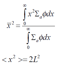
It can be calculated that L2 is equal to one-half the square of the average distance (in one dimension) between the neutron’s birth point and its absorption.
If we consider a point source of neutrons, the physical meaning of the diffusion length can be seen again by calculating the mean square distance that a neutron travels from the source to its absorption point.
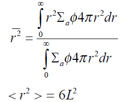
It can be calculated that:
L2 is equal to one-sixth of the square of the average distance (in all dimensions) between the neutron’s birth point (as a thermal neutron) and its absorption.
This distance must not be confused with the average distance traveled by the neutrons. The average distance traveled by the neutrons is equal to the mean free path for absorption λa = 1/Σa and is much larger than the distance measured in a straight line. This is because neutrons in the medium undergo many collisions, and they follow a very zig-zag path through the medium.
Change in the moderator and fuel temperature
The diffusion length, L2, is sensitive, especially on the change in the moderator temperature. Since diffusion in heterogeneous reactors occurs especially in the moderator, the change in the moderator temperature dominates over the change in the fuel temperature.
In short, as the moderator temperature increases, the diffusion length also increases.
The moderator temperature influences all macroscopic cross-sections (e.g.,, Σs=σs.NH2O), especially due to the thermal expansion of water, which results in a decrease in the atomic number density. The microscopic cross-sections also slightly change with temperature, but not so much in the thermal spectrum.
For the diffusion length, there are two effects. Both processes have the same direction and together cause the increase in the diffusion lengths as the temperature increases. Since the diffusion length significantly influences the thermal non-leakage probability, it is important in reactor dynamics (it influences moderator temperature feedback).
- Macroscopic cross-sections for elastic scattering reaction Σs=σs.NH2O, which significantly changes due to the thermal expansion of water. As the temperature of the core increases, the diffusion coefficient (D = 1/3.Σtr) increases.
- The macroscopic cross-section for neutron absorption also decreases as the moderator temperature increases. This is especially due to the thermal expansion of water and the changes in the microscopic cross-section (σa) for neutron absorption. As the temperature of the core increases, the absorption cross-section decreases.
Change in the boron concentration
The concentration of boric acid diluted in the primary coolant influences the diffusion length. For example, an increase in the concentration of boric acid (chemical shim) causes the addition of new absorbing material into the core, which causes an increase in the macroscopic absorption cross-section and, in turn, causes a decrease in the diffusion length.
Applicability of Diffusion Theory
Nowadays, the diffusion theory is widely used in the core design of the current Pressurized Water Reactors (PWRs) or Boiling Water Reactors (BWRs). It provides a strictly valid mathematical description of the neutron flux. Still, it must be emphasized that the diffusion equation (in fact the Fick’s law) was derived under the following assumptions:
- Infinite medium
- No sources or sinks.
- Uniform medium.
- Isotropic scattering.
- Low absorbing medium.
- Time-independent flux.
To some extent, these limitations are valid in every practical reactor. Nevertheless, the diffusion theory gives a reasonable approximation and makes accurate predictions. Nowadays, reactor core analyses and designs are often performed using nodal two-group diffusion methods. These methods are based on pre-computed assembly homogenized cross-sections, diffusion coefficients, and assembly discontinuity factors (pin factors) obtained by single assembly calculation with reflective boundary conditions (infinite lattice). Highly absorbing control elements are represented by effective diffusion theory cross-sections, which reproduce transport theory absorption rates. These pre-computed data (discontinuity factors, homogenized cross-sections, etc.) are calculated by neutron transport codes based on a more accurate neutron transport theory. In short, neutron transport theory is used to make diffusion theory work.
Two methods exist for the calculation of the pre-computed assembly cross-sections and pin factors.
- Deterministic methods that solve the Boltzmann transport equation.
- Stochastic methods are known as Monte Carlo methods that model the problem almost exactly.
These methods are very efficient and accurate when applied to the current Pressurized Water Reactors (PWRs) or Boiling Water Reactors (BWRs).
Solutions of the Diffusion Equation – Non-multiplying Systems
As was previously discussed, the diffusion theory is widely used in the core design of the current Pressurized Water Reactors (PWRs) or Boiling Water Reactors (BWRs). This section is not about such calculations but provides illustrative insights, how can be the neutron flux distributed in any diffusion medium. In this section, we will solve diffusion equations:
in various geometries that satisfy the boundary conditions discussed in the previous section.
We will start with simple systems and increase complexity gradually. The most important assumption is that all neutrons are lumped into a single energy group. They are emitted and diffuse at thermal energy (0.025 eV).
In the first section, we will deal with neutron diffusion in a non-multiplying system, i.e., in a system where fissile isotopes are missing, the fission cross-section is zero. The neutrons are emitted by an external neutron source. We will assume that the system is uniform outside the source, i.e., D and Σa are constants.
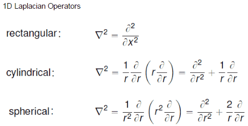
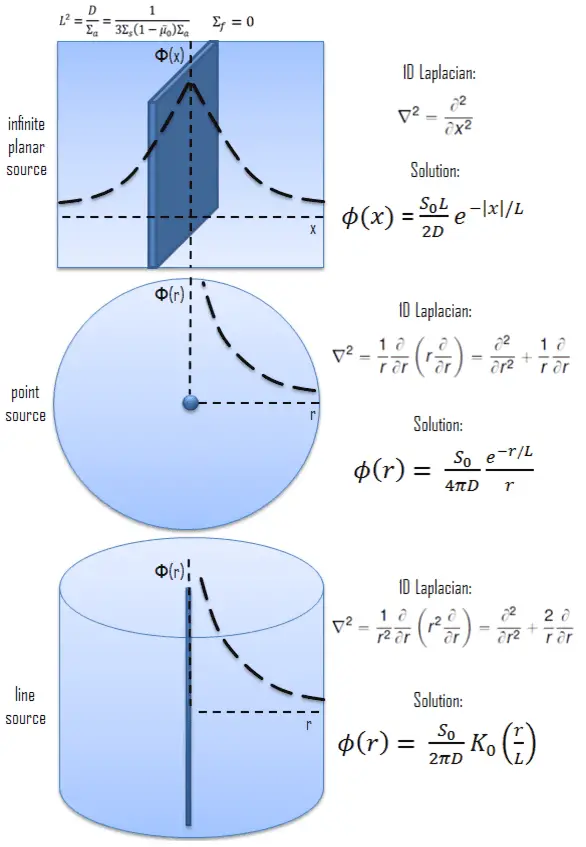
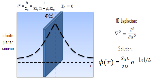 Let assume the neutron source (with strength S0) as an infinite plane source (in y-z plane geometry). In this geometry, the flux varies slowly in y and z allowing us to eliminate the y and z derivatives from ∇2. The flux is then a function of x only, and therefore the Laplacian and diffusion equation (outside the source) can be written as (everywhere except x = 0):

For x > 0, this diffusion equation has two possible solutions exp(x/L) and exp(-x/L), which give a general solution:
Φ(x) = Aexp(x/L) + Cexp(-x/L)
B is not usually used as a constant because B is reserved for a buckling parameter. To determine the coefficients A and C, we must apply boundary conditions.
From finite flux condition (0≤ Φ(x) < ∞), which required only reasonable values for the flux, it can be derived that A must be equal to zero. The term exp(x/L) goes to ∞ as x ➝∞ and therefore cannot be part of a physically acceptable solution for x > 0. The physically acceptable solution for x > 0 must then be:
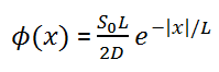
Φ(x) = Ce-x/L
where C is a constant that can be determined from the source condition at x ➝0.
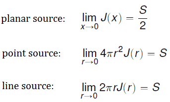
If S0 is the source strength per unit area of the plane, then the number of neutrons crossing outwards per unit area in the positive x-direction must tend to S0 /2 as x ➝0.

So that the solution may be written:
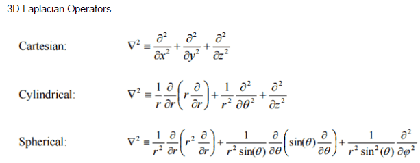
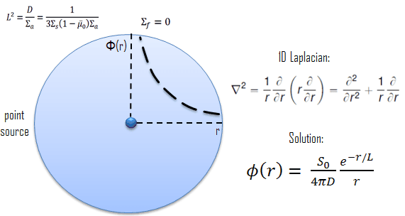 Let assume the neutron source (with strength S0) as an isotropic point source situated in spherical geometry. This point source is placed at the origin of coordinates. To solve the diffusion equation, we have to replace the Laplacian with its spherical form:

We can replace the 3D Laplacian with its one-dimensional spherical form because there is no dependence on an angle (whether polar or azimuthal). The source is assumed to be an isotropic source (there is the spherical symmetry). The flux is then a function of radius – r only, and therefore the diffusion equation (outside the source) can be written as (everywhere except r = 0):
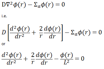
If we make the substitution Φ(r) = 1/r ψ(r), the equation simplifies to:
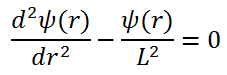
For r > 0, this differential equation has two possible solutions exp(r/L) and exp(-r/L), which give a general solution:
B is not usually used as a constant because B is reserved for a buckling parameter. To determine the coefficients A and C, we must apply boundary conditions.
To find constants A and C, we use the identical procedure as an infinite planar source. From finite flux condition (0≤ Φ(r) < ∞), which required only reasonable values for the flux, it can be derived that A must be equal to zero. The term exp(r/L)/r goes to ∞ as r ➝∞ and therefore cannot be part of a physically acceptable solution for r > 0. The physically acceptable solution for r > 0 must then be:
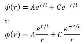
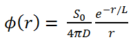
Φ(r) = Ce-r/L/r
where C is a constant that can be determined from source condition at x ➝0.
If S0 is the source strength, then the number of neutrons crossing a sphere outwards in the positive r-direction must tend to S0 as r ➝0.
So that the solution may be written:
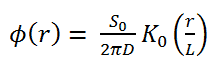
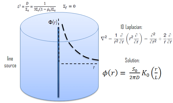 Let assume the neutron source (with strength S0) as an isotropic line source situated in an infinite cylindrical geometry. This line source is placed at r = 0. To solve the diffusion equation, we have to replace the Laplacian by its cylindrical form:
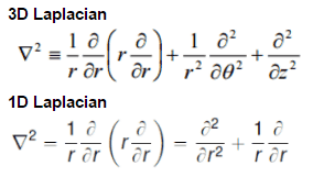
Since there is no dependence on angle Θ and z-coordinate, we can replace the 3D Laplacian with its one-dimensional form and solve the problem only in the radial direction. The source is assumed to be an isotropic source. Since the flux is a function of radius – r only, the diffusion equation (outside the source) can be written as (everywhere except r = 0):
 This differential equation is called Bessel’s equation, and it is well known to mathematicians. In this case, the solutions to the Bessel’s equation are called the modified Bessel functions (or occasionally the hyperbolic Bessel functions) of the first and second kind, Iα(x) and Kα(x), respectively.
For r > 0, this differential equation has two possible solutions, I0(r/L) and K0(r/L), the modified Bessel functions of order zero, which give a general solution:

To find constants A and C, we use the identical procedure as an infinite planar source. From finite flux condition (0≤ Φ(r) < ∞), which required only reasonable values for the flux, it can be derived that A must be equal to zero. The term I0(r/L) goes to ∞ as r ➝∞ and therefore cannot be part of a physically acceptable solution for r > 0. The physically acceptable solution for r > 0 must then be:
Φ(r) = C.K0(r/L)
where C is a constant that can be determined from the source condition at r ➝0.
If S0 is the source strength, then the number of neutrons crossing a cylinder outwards in the positive r-direction must tend to S0 as r ➝0.
So that the solution may be written:
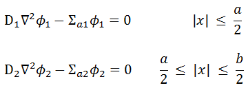
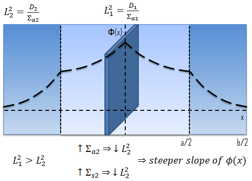
where a is the real width of zone 1 and b is the outer dimension of the diffusion environment, including the extrapolated distance. With problems involving two different diffusion media, the interface boundary conditions play a crucial role and must be satisfied:
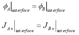
At interfaces between two different diffusion media (such as between the reactor core and the neutron reflector), on physical grounds, the neutron flux and the normal component of the neutron current must be continuous. In other words, φ and J are not allowed to show a jump.
1., 2. Interface Conditions
It must be added, as J must be continuous, the flux gradient will show a jump if the diffusion coefficients in both media differ from each other. Since the solution of these two diffusion equations requires four boundary conditions, we have to use two boundary conditions more.
3. Finite Flux Condition
The solution must be finite in those regions where the equation is valid, except perhaps at artificial singular points of a source distribution. This boundary condition can be written mathematically as:
![]() 4. Source Condition
4. Source Condition
The presence of the neutron source can be used as a boundary condition because all neutrons flowing through the bounding area of the source must come from the neutron source. This boundary condition depends on the source geometry, and for planar source can be written mathematically as:
![]()
For x > 0, these diffusion equations have the following appropriate solutions:
Φ1(x) = A1exp(x/L1) + C1exp(-x/L1)
and
Φ2(x) = A2exp(x/L2) + C2exp(-x/L2)
where the four constants must be determined with the use of the four boundary conditions. The typical neutron flux distribution in a simple two-region diffusion problem is shown in the picture below.
Solutions of the Diffusion Equation – Multiplying Systems
 In the previous section, it has been considered that the environment is non-multiplying. In a non-multiplying environment, neutrons are emitted by a neutron source situated in the center of the coordinate system and then freely diffuse through media. We are now prepared to consider neutron diffusion in the multiplying system containing fissionable nuclei (i.e., Σf ≠ 0). In this multiplying system, we will also study the spatial distribution of neutrons, but in contrast to the non-multiplying environment, these neutrons can trigger nuclear fission reactions.
This condition can be expressed conveniently in terms of the multiplication factor. The infinite multiplication factor is the ratio of the neutrons produced by fission in one neutron generation to the number of neutrons lost through absorption in the preceding neutron generation. This can be mathematically expressed as shown below.
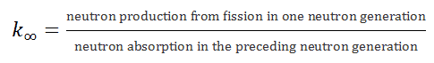
The infinite multiplication factor in a multiplying system measures the change in the fission neutron population from one neutron generation to the subsequent generation.
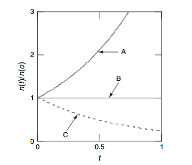
- k∞ < 1. Suppose the multiplication factor for a multiplying system is less than 1.0. In that case, the number of neutrons decreases in time (with the mean generation time), and the chain reaction will never be self-sustaining. This condition is known as the subcritical state.
- k∞ = 1. If the multiplication factor for a multiplying system is equal to 1.0, then there is no change in neutron population in time, and the chain reaction will be self-sustaining. This condition is known as the critical state.
- k∞ > 1. If the multiplication factor for a multiplying system is greater than 1.0, then the multiplying system produces more neutrons than are needed to be self-sustaining. The number of neutrons is exponentially increasing in time (with the mean generation time). This condition is known as the supercritical state.
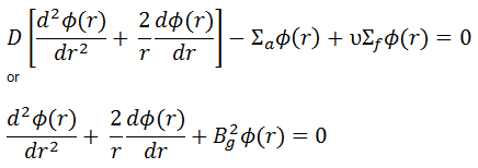
In this section, we will solve the following diffusion equation
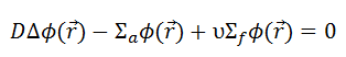
in various geometries that satisfy the boundary conditions. In this equation, ν is the number of neutrons emitted in fission, and Σf is the macroscopic cross-section of the fission reaction. Ф denotes a reaction rate. For example, the fission of 235U by thermal neutron yields 2.43 neutrons.
It must be noted that we will solve the diffusion equation without any external source. This is very important because such an equation is a linear homogeneous equation in the flux. Therefore if we find one solution of the equation, then any multiple is also a solution. This means that the absolute value of the neutron flux cannot possibly be deduced from the diffusion equation. This is totally different from problems with external sources, which determine the absolute value of the neutron flux.
We will start with simple systems (planar) and increase complexity gradually. The most important assumption is that all neutrons are lumped into a single energy group. They are emitted and diffuse at thermal energy (0.025 eV). Solutions of diffusion equations, in this case, provide illustrative insights, how can be the neutron flux distributed in a reactor core.
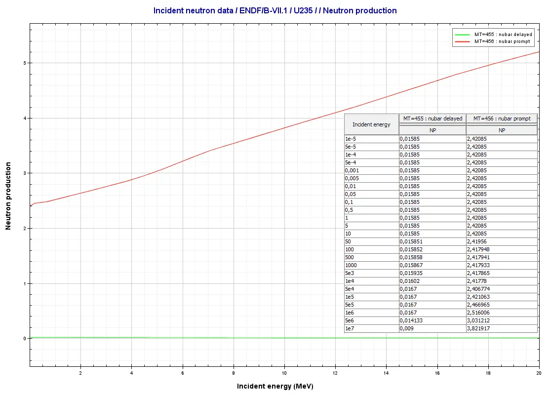
Source: JANIS (Java-based nuclear information software)
http://www.oecd-nea.org/janis/
It is known the fission neutrons are of importance in any chain-reacting system. Neutrons trigger the nuclear fission of some nuclei (235U, 238U, or even 232Th). What is crucial the fission of such nuclei produces 2, 3, or more free neutrons.
But not all neutrons are released at the same time following fission. Even the nature of the creation of these neutrons is different. From this point of view, we usually divide the fission neutrons into two following groups:
- Prompt Neutrons. Prompt neutrons are emitted directly from fission, and they are emitted within a very short time of about 10-14 seconds.
- Delayed Neutrons. Delayed neutrons are emitted by neutron-rich fission fragments that are called delayed neutron precursors. These precursors usually undergo beta decay, but a small fraction of them are excited enough to undergo neutron emission. The neutron is produced via this type of decay, and this happens orders of magnitude later compared to the emission of the prompt neutrons, which plays an extremely important role in the control of the reactor.
The most important absorption reactions are divided by the exit channel into two following reactions:
- Radiative Capture. Most absorption reactions result in the loss of a neutron coupled with the production of one or more gamma rays. This is referred to as a capture reaction, and it is denoted by σγ.
- Neutron-induced Fission Reaction. Some nuclei (fissionable nuclei) may undergo a fission event, leading to two or more fission fragments (nuclei of intermediate atomic weight) and a few neutrons. In a fissionable material, the neutron may simply be captured, or it may cause nuclear fission. For fissionable materials, we thus divide the absorption cross-section as σa = σγ+ σf.

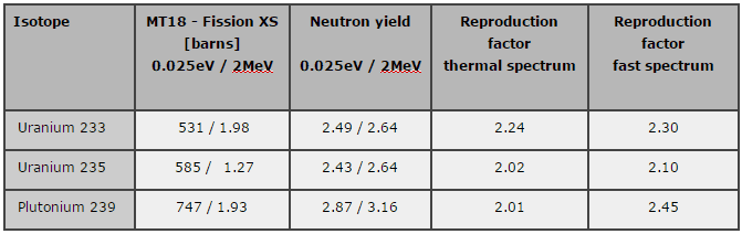
Source: JANIS 4.0
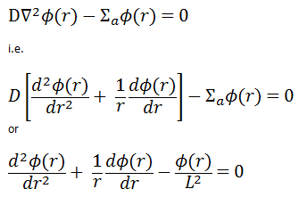
Since the neutron current is equal to zero (J = -D∇Ф, where Ф is constant), the diffusion equation in the infinite uniform multiplying system must be:
![]()
The only solution of this equation is a trivial solution, i.e., Ф = 0, unless Σa = νΣf. This equation (Σa = νΣf) is known as the criticality condition for an infinite reactor and expresses the perfect balance (critical state) between neutron absorption and neutron production. This balance must be continuously maintained to have a steady-state neutron flux.
Infinite Multiplication Factor
In this section, the infinite multiplication factor, k∞, will be defined from another point of view than in section – Nuclear Chain Reaction.
As can be seen, we can rewrite the diffusion equation in the following way, and we can define a new factor – k∞ = νΣf / Σa:
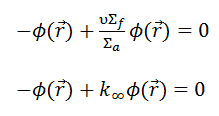
A non-trivial solution of this equation is guaranteed when k∞ = νΣf / Σa = 1. On the other hand, we have no information about the neutron flux in such a critical reactor. The neutron flux can have any value, and the critical uniform infinite reactor can operate at any power level. It should be noted this theory can be used for a reactor at low power levels, hence “zero power criticality”.
In a power reactor core, the power level does not influence the criticality of a reactor unless thermal reactivity feedbacks act (operation of a power reactor without reactivity feedbacks is between 10E-8% – 1% of rated power).
See also: Reactor Criticality
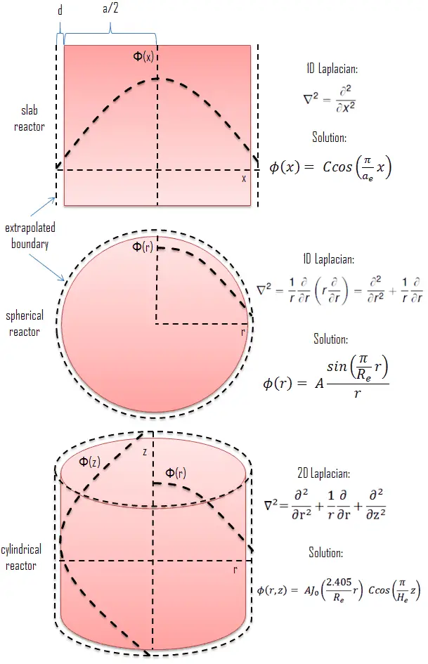
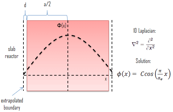 Let assume a uniform reactor (multiplying system) in the shape of a slab of physical width a in the x-direction and infinite in the y- and z-directions. This reactor is situated in the center at x=0. In this geometry, the flux does not vary in y and z allowing us to eliminate the y and z derivatives from ∇2. The flux is then a function of x only, and therefore the Laplacian and diffusion equation can be written as:
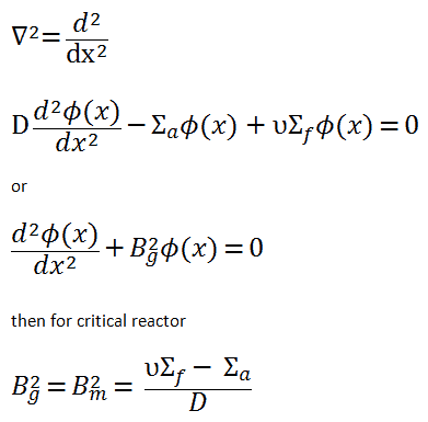
The quantity Bg2 is called the geometrical buckling of the reactor and depends only on the geometry. This term is derived from the notion that the neutron flux distribution is somehow “buckled” in a homogeneous finite reactor. It can be derived the geometrical buckling is the negative relative curvature of the neutron flux (Bg2 = ∇2Ф(x) / Ф(x)). In a small reactor, the neutron flux has more concave downward or “buckled” curvature (higher Bg2) than in a large one. This is a very important parameter, and it will be discussed in the following sections.
For x > 0, this diffusion equation has two possible solutions sin(Bgx) and cos(Bgx), which give a general solution:
Φ(x) = A.sin(Bgx) + C.cos(Bg x)
From finite flux condition (0≤ Φ(x) < ∞), which required only reasonable values for the flux, it can be derived that A must be equal to zero. The term sin(Bgx) goes to negative values as x goes to negative values, and therefore it cannot be part of a physically acceptable solution. The physically acceptable solution must then be:
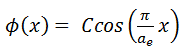
Φ(x) = C.cos(Bg x)
where Bg can be determined from the vacuum boundary condition.
The vacuum boundary condition requires the relative neutron flux near the boundary to have a slope of -1/d, i.e., the flux would extrapolate linearly to 0 at a distance d beyond the boundary. This zero flux boundary condition is more straightforward and can be written mathematically as:

If d is not negligible, the physical dimensions of the reactor are increased by d, and the extrapolated boundary is formulated with dimension ae/2 = a/2 + d. This condition can be written as Φ(a/2 + d) = Φ(ae/2) = 0.
Therefore, the solution must be Φ(ae/2) = C.cos(Bg .ae/2) = 0 and the values of geometrical buckling, Bg, are limited to Bg = nπ/a_e, where n is any odd integer. The only one physically acceptable odd integer is n=1 because higher values of n would give cosine functions which would become negative for some values of x. The solution of the diffusion equation is:
It must be added the constant C cannot be obtained from this diffusion equation because this constant gives the absolute value of neutron flux. The neutron flux can have any value, and the critical reactor can operate at any power level. It should be noted the cosine flux shape is only in the hypothetical case in a uniform homogeneous reactor at low power levels (at “zero power criticality”).
In the power reactor core (at full power operation), the neutron flux can reach, for example, about 3.11 x 10¹³ neutrons.cm-2.s-1, but this value depends significantly on many parameters (type of fuel, fuel burnup, fuel enrichment, position in fuel pattern, etc.).
The power level does not influence the criticality (keff) of a power reactor unless thermal reactivity feedbacks act (operation of a power reactor without reactivity feedbacks is between 10E-8% – 1% of rated power).
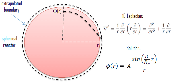 Let us assume a uniform reactor (multiplying system) in the shape of a sphere of physical radius R. The spherical reactor is situated in spherical geometry at the origin of coordinates. To solve the diffusion equation, we have to replace the Laplacian with its spherical form:
We can replace the 3D Laplacian with its one-dimensional spherical form because there is no dependence on an angle (whether polar or azimuthal). The source term is assumed to be isotropic (there is the spherical symmetry). The flux is then a function of radius – r only, and therefore the diffusion equation can be written as:
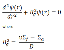
The solution of the diffusion equation is based on a substitution Φ(r) = 1/r ψ(r), that leads to an equation for ψ(r):
For r > 0, this differential equation has two possible solutions, sin(Bgr) and cos(Bgr), which give a general solution:
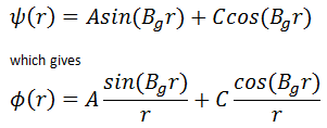
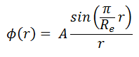
From finite flux condition (0≤ Φ(r) < ∞), which required only reasonable values for the flux, it can be derived that C must be equal to zero. The term cos(Bgr)/r goes to ∞ as r ➝0 and therefore cannot be part of a physically acceptable solution. The physically acceptable solution must then be:
Φ(r) = A sin(Bgr)/r
The vacuum boundary condition requires the relative neutron flux near the boundary to have a slope of -1/d, i.e., the flux would extrapolate linearly to 0 at a distance d beyond the boundary. This zero flux boundary condition is more straightforward and can be written mathematically as:
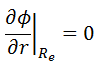
If d is not negligible, physical dimensions of the reactor are increased by d, and extrapolated boundary is formulated with dimension Re = R + d, and this condition can be written as Φ(R + d) = Φ(Re) = 0.
Therefore, the solution must be Φ(Re) = A sin(BgRe)/Re = 0, and the values of geometrical buckling, Bg, are limited to Bg = nπ/Re, where n is any odd integer. The only one physically acceptable odd integer is n=1 because higher values of n would give sine functions which would become negative for some values of x before returning to 0 at Re. The solution of the diffusion equation is:
It must be added the constant A cannot be obtained from this diffusion equation because this constant gives the absolute value of neutron flux. The neutron flux can have any value, and the critical reactor can operate at any power level. It should be noted this flux shape is only in a hypothetical case in a uniform homogeneous spherical reactor at low power levels (at “zero power criticality”).
In a power reactor core, the neutron flux can reach, for example, about 3.11 x 10¹³ neutrons.cm-2.s-1, but this value depends significantly on many parameters (type of fuel, fuel burnup, fuel enrichment, position in fuel pattern, etc.).
The power level does not influence the criticality (keff) of a power reactor unless thermal reactivity feedbacks act (operation of a power reactor without reactivity feedbacks is between 10E-8% – 1% of rated power).
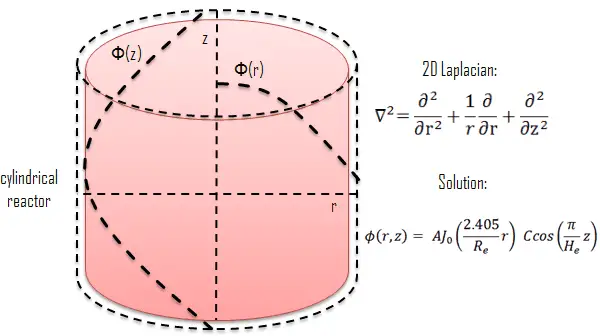 Let assume a uniform reactor (multiplying system) in the shape of a cylinder of physical radius R and height H. This finite cylindrical reactor is situated in cylindrical geometry at the origin of coordinates. To solve the diffusion equation, we have to replace the Laplacian by its cylindrical form:

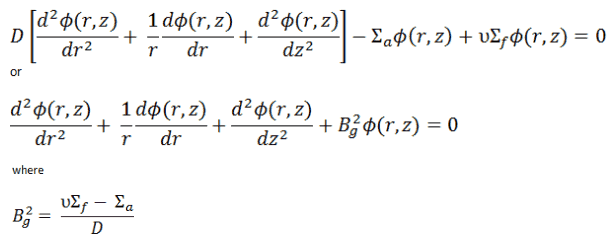
Since there is no dependence on angle Θ, we can replace the 3D Laplacian with its two-dimensional form and solve the problem in radial and axial directions. Since the flux is a function of radius – r and height – z only (Φ(r,z)), the diffusion equation can be written as:
The solution of this diffusion equation is based on the use of the separation-of-variables technique, therefore:
![]()
where R(r) and Z(z) are functions to be determined. Substituting this into the diffusion equation and dividing by R(r)Z(z), we obtain:
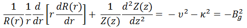
Because the first term depends only on r and the second only on z, both terms must be constants for the equation to have a solution. Suppose we take the constants to be v2 and к2. The sum of these constants must be equal to Bg2 = v2 + к2. Now we can separate variables, and the neutron flux must satisfy the following differential equations:
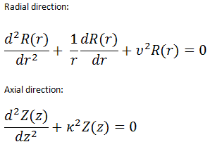
Solution for the radial direction
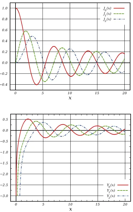 The differential equation for radial direction is called Bessel’s equation, and it is well known to mathematicians. In this case, the Bessel’s equation’s solutions are called the Bessel functions of the first and second kind, Jα(x) and Yα(x), respectively.
For r > 0, this differential equation has two possible solutions, J0(vr) and Y0(vr), the Bessel functions of order zero, which give a general solution:
![]()
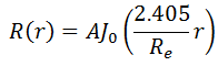
From finite flux condition (0≤ Φ(r) < ∞), which required only reasonable values for the flux, it can be derived that C must be equal to zero. The term Y0(vr) goes to -∞ as r ➝0 and therefore cannot be part of a physically acceptable solution. The physically acceptable solution must then be:
R(r) = AJ0(vr)
The vacuum boundary condition requires the relative neutron flux near the boundary to have a slope of -1/d, i.e., the flux would extrapolate linearly to 0 at a distance d beyond the boundary. This zero flux boundary condition is more straightforward and can be written mathematically as:

If d is not negligible, physical dimensions of the reactor are increased by d, and extrapolated boundary is formulated with dimension Re = R + d, and this condition can be written as Φ(R + d) = Φ(Re) = 0.
Therefore, the solution must be R(Re) = A J0(vRe) = 0. The function of J0(r) has several zeroes. The first is at r1 = 2.405, and the second at r2 = 5.6. However, because the neutron flux cannot have negative values, the only physically acceptable value for v is 2.405/Re. The solution of the diffusion equation is:
Solution for axial direction
The solution for axial direction has been solved in previous sections (Infinite Slab Reactor), and therefore it has the same solution. The solution in the axial direction is:
Solution for radial and axial directions
The full solution for the neutron flux distribution in the finite cylindrical reactor is, therefore:
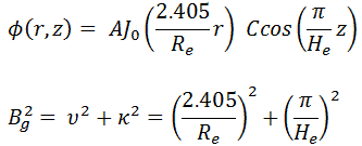
where Bg2 is the total geometrical buckling.
It must be added the constants A and C cannot be obtained from the diffusion equation because these constants give the absolute value of neutron flux. The neutron flux can have any value, and the critical reactor can operate at any power level. It should be noted this flux shape is only in a hypothetical case in a uniform homogeneous cylindrical reactor at low power levels (at “zero power criticality”).
In a power reactor core, the neutron flux can reach, for example, about 3.11 x 10¹³ neutrons.cm-2.s-1, but this value depends significantly on many parameters (type of fuel, fuel burnup, fuel enrichment, position in fuel pattern, etc.).
The power level does not influence the criticality (keff) of a power reactor unless thermal reactivity feedbacks act (operation of a power reactor without reactivity feedbacks is between 10E-8% – 1% of rated power).
See also: Reflected Reactor
Power Distribution in Conventional Reactor Cores
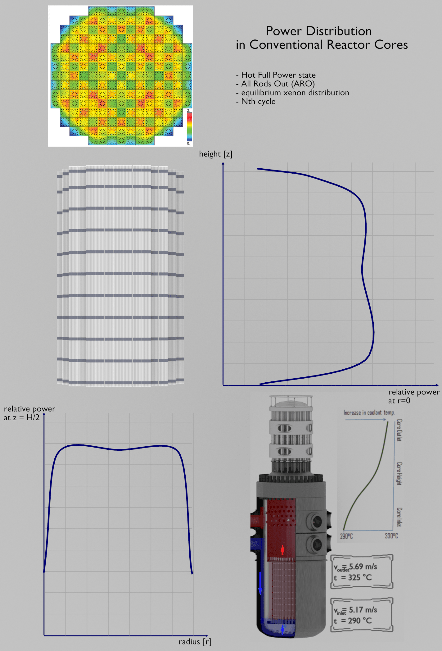
In commercial reactor cores, the flux distribution is significantly influenced by:
Heterogeneity of fuel-moderator assembly. The core’s geometry strongly influences the spatial and energy self-shielding that takes place primarily in heterogeneous reactor cores. In short, the neutron flux is not constant due to the heterogeneous geometry of the unit cell. The flux will be different in the fuel cell (lower) than in the moderator cell due to the high absorption cross-sections of fuel nuclei. This phenomenon causes a significant increase in the resonance escape probability (“p” from the four-factor formula) compared to homogeneous cores.
Reactivity Feedbacks. At power operation (i.e., above 1% of rated power), the reactivity feedbacks cause the flattening of the flux distribution because the feedbacks acts stronger on positions where the flux is higher. The neutron flux distribution in commercial power reactors depends on many other factors such as the fuel loading pattern, control rods position, and it may also oscillate within short periods (e.g.,, due to the spatial distribution of xenon nuclei). Simply, there is no cosine and J0 in the commercial power reactor at power operation.
Fuel Loading Pattern. The key feature of PWRs fuel cycles is that there are many fuel assemblies in the core. These assemblies have different multiplying properties because they may have different enrichment and different burnup. Generally, a common fuel assembly contains energy for approximately 4 years of operation at full power. Once loaded, the fuel stays in the core for 4 years, depending on the design of the operating cycle. During these 4 years, the reactor core has to be refueled. During refueling, every 12 to 18 months, some of the fuel – usually one-third or one-quarter of the core – is removed to the spent fuel pool. At the same time, the remainder is rearranged to a location in the core better suited to its remaining level of enrichment. The removed fuel (one-third or one-quarter of the core, i.e., 40 assemblies) must be replaced by a fresh fuel assembly.