Mean Generation Time with Delayed Neutrons
Mean Generation Time with Delayed Neutrons, ld, is the weighted average of the prompt generation times and a delayed neutron generation time. The delayed neutron generation time, τ, is the weighted average of mean precursor lifetimes of the six groups (or more groups) of delayed neutron precursors.
It must be noted, the true lifetime of delayed neutrons (the slowing downtime and the diffusion time) is very short compared with the mean lifetime of their precursors (ts + td << τi). Therefore τi is also equal to the mean lifetime of a neutron from the ith group, that is, τi = li, and the equation for mean generation time with delayed neutrons is the following:
ld = (1 – β).lp + ∑li . βi => ld = (1 – β).lp + ∑τi . βi
where
- (1 – β) is the fraction of all neutrons emitted as prompt neutrons
- lp is the prompt neutron lifetime
- τi is the mean precursor lifetime, the inverse value of the decay constant τi = 1/λi
- The weighted delayed generation time is given by τ = ∑τi . βi / β = 13.05 s
- Therefore the weighted decay constant λ = 1 / τ ≈ 0.08 s-1
The number, 0.08 s-1, is relatively high and has a dominating effect on reactor time response, although delayed neutrons are a small fraction of all neutrons in the core. This is best illustrated by calculating a weighted mean generation time with delayed neutrons:
ld = (1 – β).lp + ∑τi . βi = (1 – 0.0065). 2 x 10⁻⁵ + 0.085 = 0.00001987 + 0.085 ≈ 0.085
In short, the mean generation time with delayed neutrons is about ~0.1 s, rather than ~10-5 as in section Prompt Neutron Lifetime, where the delayed neutrons were omitted.
See also: Prompt Neutron Lifetime.

Example – Infinite Multiplying System Without Source and Delayed Neutrons
The simplest equation governing the neutron kinetics of the system with delayed neutrons is the point kinetics equation. This equation states that the time change of the neutron population is equal to the excess of neutron production (by fission) minus neutron loss by absorption in one mean generation time with delayed neutrons (ld). The role of ld is evident. Longer lifetimes give simply slower responses to multiplying systems.
If there are neutrons in the system at t=0, that is, if n(0) > 0, the solution of this equation gives the simplest point kinetics equation with delayed neutrons (similarly to the case without delayed neutrons):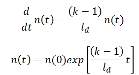 Let us consider that the mean generation time with delayed neutrons is ~0.085 and k (k∞ – neutron multiplication factor) will be step increased by only 0.01% (i.e., 10pcm or ~1.5 cents), that is k∞=1.0000 will increase to k∞=1.0001.
It must be noted such reactivity insertion (10pcm) is very small in the case of LWRs. The reactivity insertions of the order of one pcm are for LWRs practically unrealizable. In this case, the reactor period will be:
T = ld / (k∞-1) = 0.085 / (1.0001-1) = 850s
This is a very long period. In ~14 minutes, the reactor’s neutron flux (and power) would increase by a factor of e = 2.718. This is a completely different dimension of the response on reactivity insertion compared to the case without delayed neutrons, where the reactor period was 1 second.
Reactors with such kinetics would be quite easy to control. From this point of view, it may seem that reactor control will be quite a boring affair. It will not! The presence of delayed neutrons entails many, many specific phenomena that will be described in later chapters.
Interactive chart – Infinite Multiplying System Without Source and with Delayed Neutrons
Press the “clear and run” button and try to increase the power of the reactor.
Compare the response of the reactor with the case of Infinite Multiplying System Without Source and without Delayed Neutrons (or set the β = 0).