Reactor Dynamics

Prompt and Delayed Neutrons

It is known that fission neutrons are of importance in any chain-reacting system. Neutrons trigger the nuclear fission of some nuclei (²³⁵U, ²³⁸U, or even ²³²Th). What is crucial the fission of such nuclei produces 2, 3, or more free neutrons.

But not all neutrons are released at the same time following fission. Even the nature of the creation of these neutrons is different. From this point of view, we usually divide the fission neutrons into two following groups:

• Prompt Neutrons. Prompt neutrons are emitted directly from fission, and they are emitted within a very short time of about 10^-14 seconds.
• Delayed Neutrons. Delayed neutrons are emitted by neutron-rich fission fragments that are called delayed neutron precursors. These precursors usually undergo beta decay, but a small fraction of them are excited enough to undergo neutron emission. The fact the neutron is produced via this type of decay, and this happens orders of magnitude later compared to the emission of the prompt neutrons, plays an extremely important role in the control of the reactor.

Key Characteristics of Prompt Neutrons

• Prompt neutrons are emitted directly from fission, and they are emitted within a very short time of about 10^-14 seconds.

• Most of the neutrons produced in fission are prompt neutrons – about 99.9%.

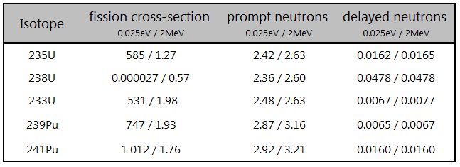
• For example, fission of ²³⁵U by thermal neutron yields 2.43 neutrons, of which 2.42 neutrons are prompt neutrons, and 0.01585 neutrons are the delayed neutrons.

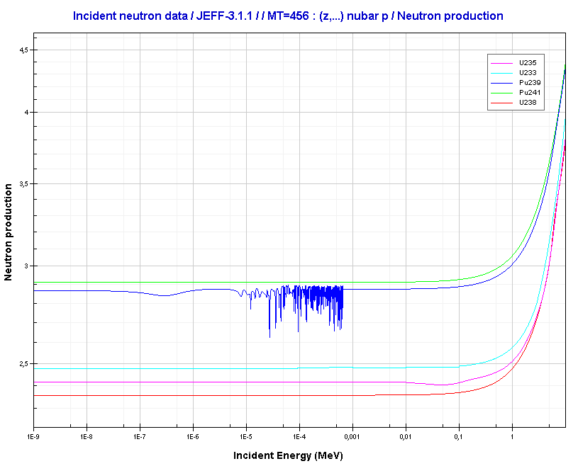
• The production of prompt neutrons slightly increases with incident neutron energy.

• Almost all prompt fission neutrons have energies between 0.1 MeV and 10 MeV.

• The mean neutron energy is about 2 MeV. The most probable neutron energy is about 0.7 MeV.

• In reactor design, the prompt neutron lifetime (PNL) belongs to key neutron-physical characteristics of the reactor core.

• Its value depends especially on the type of the moderator and on the energy of the neutrons causing fission.

• In an infinite reactor (without escape), prompt neutron lifetime is the sum of the slowing down time and the diffusion time.

• In LWRs, the PNL increases with the fuel burnup.

• The typical prompt neutron lifetime in thermal reactors is on the order of 10^-4 seconds.

• The typical prompt neutron lifetime in fast reactors is on the order of 10^-7 seconds.

Key Characteristics of Delayed Neutrons

• The presence of delayed neutrons is perhaps the most important aspect of the fission process from the viewpoint of reactor control.

• Delayed neutrons are emitted by neutron-rich fission fragments that are called delayed neutron precursors.

• These precursors usually undergo beta decay, but a small fraction of them are excited enough to undergo neutron emission.

• The emission of neutrons happens orders of magnitude later compared to the emission of the prompt neutrons.

• About 240 n-emitters are known between ⁸He and ²¹⁰Tl, about 75 of them are in the non-fission region.

• To simplify reactor kinetic calculations, it is suggested to group together the precursors based on their half-lives.

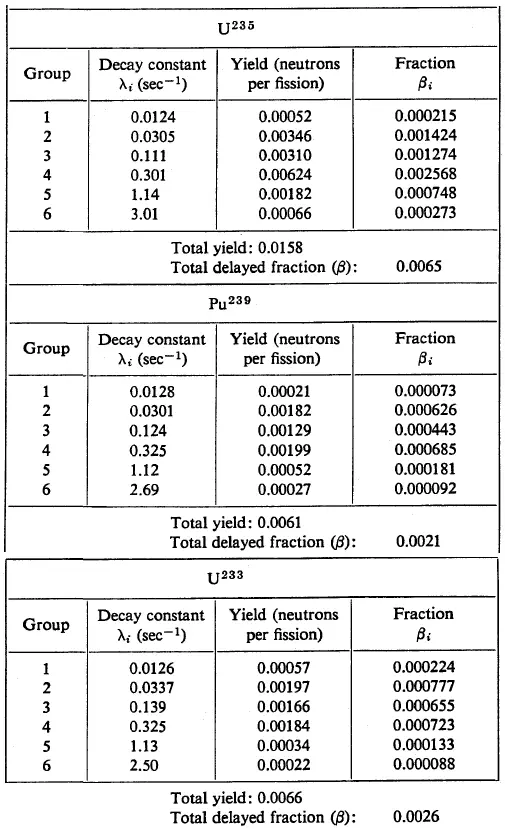
• Therefore delayed neutrons are traditionally represented by six delayed neutron groups.

• Neutrons can also be produced in (γ, n) reactions (especially in reactors with heavy water moderators), and therefore they are usually referred to as photoneutrons. Photoneutrons are usually treated no differently than delayed neutrons in the kinetic calculations.

• The total yield of delayed neutrons per fission, v_d, depends on:
  • Isotope that is fissioned.
  • Energy of a neutron that induces fission.

• Variation among individual group yields is much greater than variation among group periods.

• In reactor kinetic calculations, it is convenient to use relative units usually referred to as delayed neutron fraction (DNF).

• At the steady-state condition of criticality, with k_eff = 1, the delayed neutron fraction is equal to the precursor yield fraction β.

• In LWRs, the β decreases with fuel burnup. This is due to isotopic changes in the fuel.

• Delayed neutrons have initial energy between 0.3 and 0.9 MeV with an average energy of 0.4 MeV.

• Depending on the type of the reactor, and their spectrum, the delayed neutrons may be more (in thermal reactors) or less effective than prompt neutrons (in fast reactors). To include this effect into the reactor kinetic calculations, the effective delayed neutron fraction – β_eff must be defined.

• The effective delayed neutron fraction is the product of the average delayed neutron fraction and the importance factor β_eff = β . I.

• The weighted delayed generation time is given by τ = ∑_iτ_i . β_i / β = 13.05 s, therefore the weighted decay constant λ = 1 / τ ≈ 0.08 s^-1.

• The mean generation time with delayed neutrons is about ~0.1 s, rather than ~10^-5 as in section Prompt Neutron Lifetime, where the delayed neutrons were omitted.

• Their presence completely changes the dynamic time response of a reactor to some reactivity change, making it controllable by control systems such as the control rods.

Point Kinetics Equations

As we have seen in previous chapters, the number of neutrons is multiplied by a factor k_eff from one neutron generation to the next; therefore, the multiplication environment (nuclear reactor) behaves like the exponential system, which means the power increase is not linear, but it is exponential.

It is obvious the effective multiplication factor in a multiplying system is a measure of the change in the fission neutron population from one neutron generation to the subsequent generation.

• k_eff < 1. Suppose the multiplication factor for a multiplying system is less than 1.0. In that case, the number of neutrons decreases in time (with the mean generation time), and the chain reaction will never be self-sustaining. This condition is known as the subcritical state.

• k_eff = 1. Suppose the multiplication factor for a multiplying system is equal to 1.0, then there is no change in neutron population in time, and the chain reaction will be self-sustaining. This condition is known as the critical state.

• k_eff > 1. Suppose the multiplication factor for a multiplying system is greater than 1.0, then the multiplying system produces more neutrons than are needed to be self-sustaining. The number of neutrons is exponentially increasing in time (with the mean generation time). This condition is known as the supercritical state.

But we have not yet discussed the duration of a neutron generation, which means how many times in one second we have to multiply the neutron population by a factor k_eff. This time determines the speed of the exponential growth. But as was written, there are different types of neutrons: prompt neutrons and delayed neutrons, which completely change the kinetic behavior of the system. Therefore such a discussion will be not trivial.

To study the kinetic behavior of the system, engineers usually use point kinetics equations. The name point kinetics is used because, in this simplified formalism, the neutron flux shape and the neutron density distribution are ignored. The reactor is therefore reduced to a point. In the following section, we will introduce the point kinetics, and we start with point kinetics in its simplest form.

See also: Point Kinetics Equation

Simple Point Kinetics Equation with Delayed Neutrons

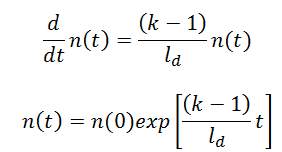
The simplest equation governing the neutron kinetics of the system with delayed neutrons is the simple point kinetics equation with delayed neutrons. This equation states that the time change of the neutron population is equal to the excess of neutron production (by fission) minus neutron loss by absorption in one mean generation time with delayed neutrons (l_d).

l_d = (1 – β).l_p + ∑l_i . β_i => l_d = (1 – β).l_p + ∑τ_i . β_i

where

• (1 – β) is the fraction of all neutrons emitted as prompt neutrons
• l_p is the prompt neutron lifetime
• τ_i is the mean precursor lifetime, the inverse value of the decay constant τ_i = 1/λ_i
• The weighted delayed generation time is given by τ = ∑τ_i . β_i / β = 13.05 s
• Therefore the weighted decay constant λ = 1 / τ ≈ 0.08 s^-1

The number, 0.08 s^-1, is relatively high and has a dominating effect on reactor time response, although delayed neutrons are a small fraction of all neutrons in the core. This is best illustrated by calculating a weighted mean generation time with delayed neutrons:

l_d = (1 – β).l_p + ∑τ_i . β_i = (1 – 0.0065). 2 x 10^-5 + 0.085 = 0.00001987 + 0.085 ≈ 0.085

In short, the mean generation time with delayed neutrons is about ~0.1 s, rather than ~10^-5 as in section Prompt Neutron Lifetime, where the delayed neutrons were omitted.

The role of l_d is evident. Longer lifetimes give simply slower responses of multiplying systems. The role of reactivity (k_eff – 1) is also evident. Higher reactivity gives a larger response of the multiplying system.

If there are neutrons in the system at t=0, that is, if n(0) > 0, the solution of this equation gives the simplest point kinetics equation with delayed neutrons (similarly to the case without delayed neutrons):

Example:

Let us consider that the mean generation time with delayed neutrons is ~0.085, and k (k_∞ – neutron multiplication factor) will be step increased by only 0.01% (i.e., 10pcm or ~1.5 cents); that is, k_∞=1.0000 will increase to k_∞=1.0001.

It must be noted such reactivity insertion (10pcm) is very small in the case of LWRs (e.g., one step by control rods). The reactivity insertions of the order of one pcm are for LWRs practically unrealizable. In this case, the reactor period will be:

T = l_d / (k_∞-1) = 0.085 / (1.0001-1) = 850s

This is a very long period. In ~14 minutes, the neutron flux (and power) in the reactor would increase by a factor of e = 2.718. This is completely different dimension of the response on reactivity insertion in comparison with the case without the presence of delayed neutrons, where the reactor period was 1 second.

Six Groups of Delayed Neutrons

Reactor-kinetic calculations considering such several initial conditions would be correct, but it also would be very complicated. Therefore G. R. Keepin and his co-workers suggested grouping together the precursors based on their half-lives. Therefore delayed neutrons are traditionally represented by six delayed neutron groups, whose yields and decay constants (λ) are obtained from nonlinear least-squares fits experimental measurements. This model has the following disadvantages:

• All constants for each group of precursors are empirical fits to the data.

• They cannot be matched with decay constants of specific precursors.

• These constants are different for each fissionable nuclide.

• These constants also change with the neutron energy spectrum.

Although this six-group parameterization still satisfies the requirements of commercial organizations, higher accuracy of the delayed neutron yields and a better energy resolution in the delayed neutron spectra is desired.

It was recognized that the half-lives in the six-group structure do not accurately reproduce the asymptotic die-away time constants associated with the three longest-lived dominant precursors: ⁸⁷Br, ¹³⁷I, and ⁸⁸Br.

This model may be insufficient, especially in the case of epithermal reactors, because virtually all delayed neutron activity measurements have been performed for fast or thermal-neutron-induced fission. In the case of fast reactors, in which the nuclear fission of six fissionable isotopes of uranium and plutonium is important, the accuracy and energy resolution may play an important role.

Effective Delayed Neutron Fraction – βeff

See also: Delayed Neutron Fraction

See also: Effective Delayed Neutron Fraction – βeff

The delayed neutron fraction, β, is the fraction of delayed neutrons in the core at creation, that is, at high energies. But in the case of thermal reactors, the fission can be initiated mainly by a thermal neutron. Thermal neutrons are of practical interest in the study of thermal reactor behavior. The effective delayed neutron fraction usually referred to as β_eff, is the same fraction at thermal energies.

The effective delayed neutron fraction reflects the ability of the reactor to thermalize and utilize each neutron produced. The β is not the same as the β_eff due to the fact delayed neutrons do not have the same properties as prompt neutrons released directly from fission. In general, delayed neutrons have lower energies than prompt neutrons. Prompt neutrons have initial energy between 1 MeV and 10 MeV, with an average energy of 2 MeV. Delayed neutrons have initial energy between 0.3 and 0.9 MeV with an average energy of 0.4 MeV.

Therefore in thermal reactors, a delayed neutron traverses a smaller energy range to become thermal, and it is also less likely to be lost by leakage or by parasitic absorption than is the 2 MeV prompt neutron. On the other hand, delayed neutrons are also less likely to cause fast fission because their average energy is less than the minimum required for fast fission to occur.

These two effects (lower fast fission factor and higher fast non-leakage probability for delayed neutrons) tend to counteract each other and form a term called the importance factor (I). The importance factor relates the average delayed neutron fraction to the effective delayed neutron fraction. As a result, the effective delayed neutron fraction is the product of the average delayed neutron fraction and the importance factor.

β_eff = β . I

The delayed and prompt neutrons have a difference in their effectiveness in producing a subsequent fission event. Since the energy distribution of the delayed neutrons also differs from group to group, the different groups of delayed neutrons will also have different effectiveness. Moreover, a nuclear reactor contains a mixture of fissionable isotopes. Therefore, in some cases, the importance factor is insufficient, and an importance function must be defined.

For example:

In a small thermal reactor with highly enriched fuel, the increase in fast non-leakage probability will dominate the decrease in the fast fission factor, and the importance factor will be greater than one.

In a large thermal reactor with low enriched fuel, the decrease in the fast fission factor will dominate the increase in the fast non-leakage probability, and the importance factor will be less than one (about 0.97 for a commercial PWR).

In large fast reactors, the decrease in the fast fission factor will also dominate the increase in the fast non-leakage probability, and the β_eff is less than β by about 10%.

Mean Generation Time with Delayed Neutrons

Mean Generation Time with Delayed Neutrons, l_d, is the weighted average of the prompt generation times and a delayed neutron generation time. The delayed neutron generation time, τ, is the weighted average of mean precursor lifetimes of the six groups (or more groups) of delayed neutron precursors.

It must be noted, the true lifetime of delayed neutrons (the slowing down time and the diffusion time) is very short compared with the mean lifetime of their precursors (t_s + t_d << τ_i). Therefore τ_i is also equal to the mean lifetime of a neutron from the ith group, that is, τ_i = l_i, and the equation for mean generation time with delayed neutrons is the following:

l_d = (1 – β).l_p + ∑l_i . β_i => l_d = (1 – β).l_p + ∑τ_i . β_i

where

• (1 – β) is the fraction of all neutrons emitted as prompt neutrons
• l_p is the prompt neutron lifetime
• τ_i is the mean precursor lifetime, the inverse value of the decay constant τ_i = 1/λ_i
• The weighted delayed generation time is given by τ = ∑τ_i . β_i / β = 13.05 s
• Therefore the weighted decay constant λ = 1 / τ ≈ 0.08 s^-1

The number, 0.08 s^-1, is relatively high and has a dominating effect on reactor time response, although delayed neutrons are a small fraction of all neutrons in the core. This is best illustrated by calculating a weighted mean generation time with delayed neutrons:

l_d = (1 – β).l_p + ∑τ_i . β_i = (1 – 0.0065). 2 x 10^-5 + 0.085 = 0.00001987 + 0.085 ≈ 0.085

In short, the mean generation time with delayed neutrons is about ~0.1 s, rather than ~10-5 as in section Prompt Neutron Lifetime, where the delayed neutrons were omitted.

Effect of Delayed Neutrons on Reactor Control

Despite the fact the number of delayed neutrons per fission neutron is quite small (typically below 1%) and thus does not contribute significantly to the power generation, they play a crucial role in the reactor control and are essential from the point of view of reactor kinetics and reactor safety. Their presence completely changes the dynamic time response of a reactor to some reactivity change, making it controllable by control systems such as the control rods.

Delayed neutrons allow to operate a reactor in a prompt subcritical, delayed critical condition. All power reactors are designed to operate in delayed critical conditions and are provided with safety systems to prevent them from ever achieving prompt criticality.

For typical PWRs, the prompt criticality occurs after positive reactivity insertion of β_eff(i.e., k_eff ≈ 1.006 or ρ = +600 pcm). In power reactors, such a reactivity insertion is practically impossible to insert (in case of normal and abnormal operation), especially when a reactor is in power operation mode and a reactivity insertion causes heating of a reactor core. Due to the presence of reactivity feedbacks, the positive reactivity insertion is counterbalanced by the negative reactivity from moderator and fuel temperature coefficients. The presence of delayed neutrons is of importance also from this point of view because they provide time also to reactivity feedbacks to react on undesirable reactivity insertion.

Interactive chart – Infinite Multiplying System Without Source and Delayed Neutrons

Press the “clear and run” button and try to increase the power of the reactor.

Compare the response of the reactor with the case of Infinite Multiplying System Without Source and without Delayed Neutrons (or set the β = 0).

Inhour Equation

If the reactivity is constant, the model of point kinetics equations contains a set (1 + 6) of linear ordinary differential equations with constant coefficient and can be solved analytically. Solution of six-group point kinetics equations with Laplace transformation leads to the relation between the reactivity and the reactor period. This relation is known as the inhour equation (which comes from an inverse hour, when it was used as a unit of reactivity that corresponded to e-fold neutron density change during one hour) may be derived.

General Form:

The point kinetics equations may be solved for the case of an initially critical reactor without an external source in which the properties are changed at t = 0 in such a way as to introduce a step reactivity ρ₀ which is then constant over time. The system of coupled first-order differential equations can be solved with Laplace transformation or by trying the solution n(t) = A.exp(s.t) (equation for the neutron flux) and C_i(t) = C_i,0.exp(s.t) (equations for the density of precursors).

Substitution of these assumed exponential solutions in the equation for precursors gives the relation between the coefficients of the neutron density and the precursors.

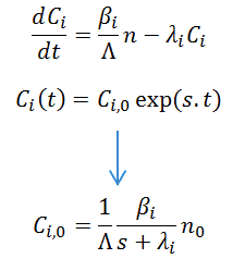
The subsequent substitution in the equation for neutron density yields an equation for s, which after some manipulation can be written as:

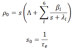
This equation is known as the inhour equation since the constants of s_{0 – 6} were originally determined in inverse hours. For a given value of the reactivity ρ, the associated values of s_{0 – 6} are determined with this equation. The following figure shows the relation between ρ and roots s graphically. This figure shows that for a given value of ρ, seven solutions exist for s. The figure indicates that for positive reactivity, only s₀ is positive. The remaining terms rapidly die away, yielding an asymptotic solution in the form:

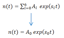
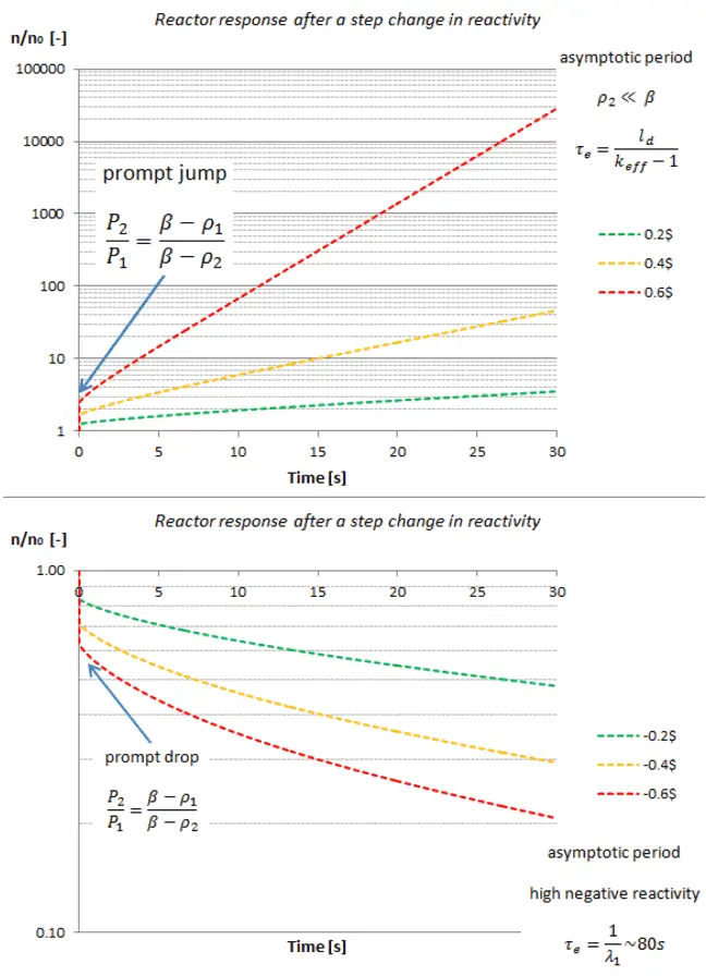
where s₀ = 1/τ_e is the stable reactor period or asymptotic period of the reactor. This root, s₀, is positive for ρ > 0 and negative for ρ < 0; therefore, this root describes the reactor response, which is lasting after the transition phenomena have died out. The figure also shows that a negative reactivity leads to a negative period: All of the s_i are negative, but the root s₀ will die away more slowly than the others. Thus the solution n(t) = A₀exp(s₀t) is valid for positive as well as negative reactivity insertions.

To determine the reactivity required to produce a given period, a plot of ρ vs. τ_e must be constructed using the delayed neutron data for a particular fissionable isotope or a mix of isotopes, and for a given prompt generation time. To determine the stable reactor period, which results from a given reactivity insertion, it is convenient to use the following form of an inhour equation.

Reactor Period Form of Inhour Equation

where:

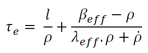
l = prompt neutron lifetime

β_eff = effective delayed neutron fraction

λ_eff = effective delayed neutron precursor decay constant

τ_e = reactor period

ρ = reactivity

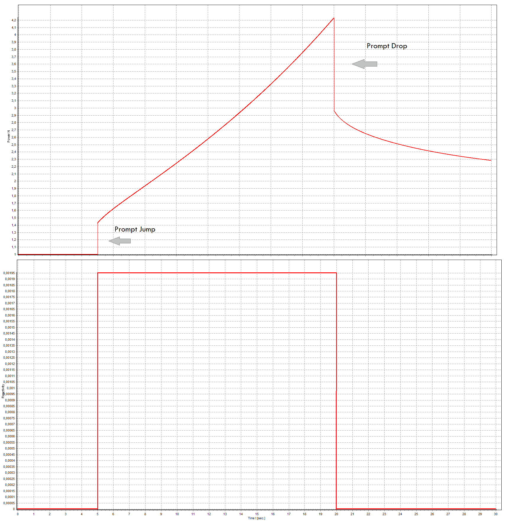
The first term in this formula is the prompt term and it causes that the positive reactivity insertion is followed immediately by an immediate power increase called the prompt jump. This power increase occurs because the rate of production of prompt neutrons changes immediately as the reactivity is inserted. After the prompt jump, the rate of change of power cannot increase any more rapidly than the built-in time delay the precursor half-lives allow. Therefore the second term in this formula is called the delayed term. The presence of delayed neutrons causes the power rise to be controllable, and the reactor can be controlled by control rods or another reactivity control mechanism.

Reactor Period and Startup Rate

reactivity is not directly measurable, and therefore most power reactors procedures do not refer to it, and most technical specifications do not limit it. Instead, they specify a limiting rate of neutron power rise (measured by excore detectors), commonly called a startup rate (especially in the case of PWRs).

The reactor startup rate is defined as the number of factors of ten that power changes in one minute. Therefore the units of SUR are powers of ten per minute or decades per minute (dpm). The relationship between reactor power and startup rate is given by the following equation:

n(t) = n(0).10^SUR.t

where:
SUR = reactor startup rate [dpm – decades per minute]
t = time during reactor transient [minute]

The higher the value of SUR, the more rapid the change in reactor power. The startup rate may be positive or negative. If SUR is positive, reactor power is increasing. If SUR is negative, reactor power is decreasing. The relationship between reactor period and startup rate is given by the following equations:

Example:

Suppose k_eff = 1.0005 in a reactor with a generation time l_d = 0.01s. For this state calculate the reactor period – τ_e, doubling time – DT and the startup rate (SUR).
ρ = 1.0005 – 1 / 1.0005 = 50 pcm

τ_e = l_d / k-1 = 0.1 / 0.0005 = 200 s

DT = τ_e . ln2 = 139 s

SUR = 26.06 / 200 = 0.13 dpm

See also: Inhour Equation

Reactivity

In the preceding chapters, the classification of states of a reactor according to the effective multiplication factor – k_eff was introduced. The effective multiplication factor – k_eff is a measure of the change in the fission neutron population from one neutron generation to the subsequent generation. But sometimes, it is convenient to define the change in the k_eff alone, the change in the state, from the criticality point of view.

For these purposes reactor physics use a term called reactivity rather than k_eff to describe the change in the state of the reactor core. The reactivity (ρ or ΔK/K) is defined in terms of k_eff by the following equation:

From this equation, it may be seen that ρ may be positive, zero, or negative. The reactivity describes the deviation of an effective multiplication factor from unity. For critical conditions, the reactivity is equal to zero. The larger the absolute value of reactivity in the reactor core, the further the reactor is from criticality. In fact, the reactivity may be used as a measure of a reactor’s relative departure from criticality.

It must be noted the reactivity can also be calculated according to another formula.

This formula is widely used in neutron diffusion or neutron transport codes. The advantage of this reactivity is obvious, it is a measure of a reactor’s relative departure not only from criticality (k_eff = 1), but it can be related to any sub or supercritical state (ln(k₂ / k₁)). Another important feature arises from the mathematical properties of the logarithm. The logarithm of the division of k₂ and k₁ is the difference of the logarithm of k₂ and the logarithm of k₁. ln(k₂ / k₁) = ln(k₂) – ln(k₁). This feature is important in the case of addition and subtraction of various reactivity changes.

See more: D.E.Cullen, Ch.J.Clouse, R.Procassini, R.C.Little. Static and Dynamic Criticality: Are They Different?. Lawrence Livermore National Laboratory. UCRL-TR-201506. 11/2003.

See more about reactivity.

Reactivity Coefficients – Reactivity Feedbacks

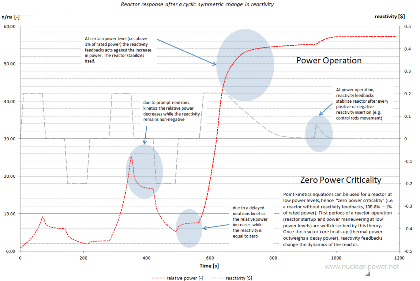
Up to this point, we have discussed the response of the neutron population in a nuclear reactor to an external reactivity input. There was applied an assumption that the level of the neutron population does not affect the properties of the system, especially that the neutron power (power generated by chain reaction) is sufficiently low that the reactor core does not change its temperature (i.e., reactivity feedbacks may be neglected). For this reason, such treatments are frequently referred to as zero-power kinetics.

However, in an operating power reactor, the neutron population is always large enough to generated heat. In fact, it is the main purpose of power reactors to generate a large amount of heat. This causes the system’s temperature to change, and material densities change as well (due to the thermal expansion).

Because macroscopic cross-sections are proportional to densities and temperatures, the neutron flux spectrum also depends on the density of the moderator; these changes, in turn, will produce some changes in reactivity. These changes in reactivity are usually called reactivity feedbacks and are characterized by reactivity coefficients. This is a very important area of reactor design because the reactivity feedbacks influence the stability of the reactor. For example, reactor design must assure that under all operating conditions, the temperature feedback will be negative.

Example: Change in the moderator temperature.

Negative feedback as the moderator temperature effect influences the neutron population in the following way. If the temperature of the moderator is increased, negative reactivity is added to the core. This negative reactivity causes reactor power to decrease. As the thermal power decreases, the power coefficient acts against this decrease, and the reactor returns to the critical condition. The reactor power stabilizes itself. In terms of multiplication factor, this effect is caused by significant changes in the resonance escape probability and in the total neutron leakage (or in the thermal utilization factor when the chemical shim is used).

Reactivity Coefficients

To describe the influence of all these processes on reactivity, one defines the reactivity coefficient α. A reactivity coefficient is defined as the change of reactivity per unit change in some operating parameter of the reactor. For example:

α = ^dρ⁄_dT

The amount of reactivity, which is inserted to a reactor core by a specific change in an operating parameter, is usually known as the reactivity effect and is defined as:

dρ = α . dT

The reactivity coefficients that are important in power reactors (PWRs) are:

• Moderator Temperature Coefficient – MTC
• Fuel Temperature Coefficient or Doppler Coefficient
• Pressure Coefficient
• Void Coefficient

As can be seen, there are not only temperature coefficients that are defined in reactor dynamics. In addition to these coefficients, there are two other coefficients:

• Total Power Coefficient
• Boron Coefficient

The total power coefficient is the combination of various effects and is commonly used when reactors are at power conditions. It is due to the fact, at power conditions it is difficult to separate the moderator effect from the fuel effect and the void effect as well. All these coefficients will be described in following separate sections. The reactivity coefficients are of importance in safety of each nuclear power plant which is declared in the Safety Analysis Report (SAR).

Feedback Delay – Time Constants

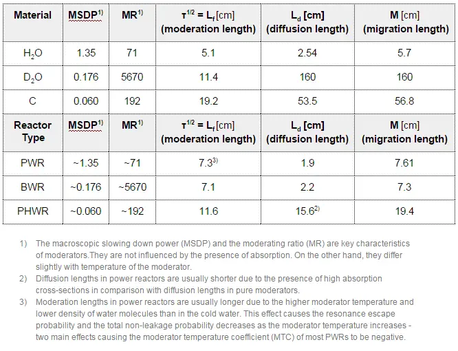
In physics and engineering, the time constant is the parameter characterizing the response to a step input of a first-order, linear time-invariant system. The time constant is usually denoted by the Greek letter τ (tau). It is obvious that thermal time constants, which characterize the time required to warm an object by another object, are of importance for reactor stability. In general, the heat transfer from the body to the ambient at a given time is proportional to the temperature difference between the body and the ambient. The time constants that determine the time delays for reactivity feedbacks depend on the specific reactor design. For LWRs, the following time constants are usual:

• The time constant for heating fuel is almost zero; therefore, the fuel temperature coefficient is effective almost instantaneously.
• The time constant for heat transfer out of a fuel pin varies from a few tenths to a few tens of seconds. The time for heat to be transferred to the moderator is usually measured in seconds (~5s). The presence of the surface film increases the time constant for the fuel element.
• The time constant for equalization of temperatures within the primary loop depends strongly on the length of primary piping and the flow velocity. It is usually measured in seconds (<10s)

Knowledge of delays of reactivity feedbacks is very important in the study of reactor transients. A large reactivity insertion will cause a reactor to go on such a short period that the power changes significantly over a short time span compared to the number of seconds needed to transfer heat from fuel to coolant. Especially in the case of all reactivity-initiated accidents (RIA), over short time spans, the amount of heat transferred to the coolant is not enough to increase its temperature appreciably. Therefore, the fuel temperature coefficient will be the first and the most important feedback that will compensate for the inserted positive reactivity. The time for heat to be transferred to the moderator is usually measured in seconds, while the fuel temperature coefficient is effective almost instantaneously. Therefore this coefficient is also called the prompt temperature coefficient because it causes an immediate response to changes in fuel temperature.

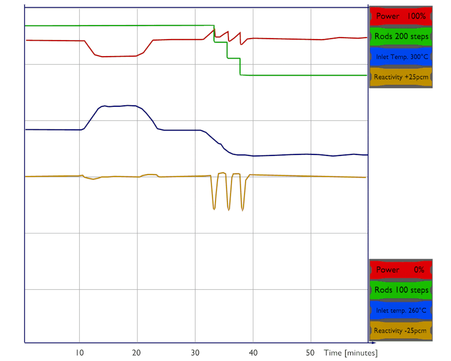
Point Dynamics Equations

A simple point dynamics model is based on point kinetics equations, but here we should take into account the influence of the fuel and the moderator temperature on the reactivity. We assume there are no other feedbacks, and therefore this simple model can be applied only on PWRs. For example, the void coefficient is neglected here. In systems with boiling conditions, such as boiling water reactors (BWR), the void coefficient is of prime importance during reactor operation.

Thus, the simplest point dynamics model of PWR should take into consideration the time variations of the fuel and coolant temperature. The point dynamics model consist of the following equations:

• The first equation is the equation for neutrons. The first term on the right-hand side is the production of prompt neutrons in the present generation, minus the total number of neutrons in the preceding generation. The second term is the production of delayed neutrons in the present generation.
• The second equation is the equation for precursors. There is a balance between the production of the precursors of i-th group and their decay after the decay constant λ_i. As can be seen, the decay rate of precursors is the radioactivity rate (λ_iC_i), and the rate of production is proportional to the number of neutrons times β_i, which is defined as the fraction of the neutrons which appear as delayed neutrons in the ith group.
• The third equation expresses the dependence of the reactivity on various parameters. But in this case, there is a dependence on the coolant and the fuel temperature only. ρ₀ is the initial reactivity, whereas ρ_C (t) is time-dependent reactivity inserted by a reactor control system (e.g., by control rods or by boron dilution). This is the feedback equation.
• The equations of the heat balance for fuel and coolant are interconnected via h(T_F – T_C), which represents the heat transfer from the fuel into the coolant. In these equations, m_F and m_C are the mass of fuel and coolant in the core, respectively, c_pF and c_pC are specific heat capacities of fuel and coolant, h is the heat transfer coefficient between fuel and coolant, m_C dotted is the coolant mass flow rate [kg/s] and T_C and T_C,in are the average and inlet coolant temperature, respectively.

To solve the point dynamics equations, it is necessary to specify the initial conditions, like in the case of point kinetics.

See also: Reactor Stability

What means under and over-moderated reactor?