As we have seen in previous chapters, the number of neutrons is multiplied by a factor keff from one neutron generation to the next. Therefore, the multiplication environment (nuclear reactor) behaves like an exponential system, which means the power increase is not linear but exponential.
 The effective multiplication factor in a multiplying system measures the change in the fission neutron population from one neutron generation to the subsequent generation.
- keff < 1. Suppose the multiplication factor for a multiplying system is less than 1.0. In that case, the number of neutrons decreases in time (with the mean generation time), and the chain reaction will never be self-sustaining. This condition is known as the subcritical state.
- keff = 1. If the multiplication factor for a multiplying system is equal to 1.0, then there is no change in neutron population in time, and the chain reaction will be self-sustaining. This condition is known as the critical state.
- keff > 1. If the multiplication factor for a multiplying system is greater than 1.0, then the multiplying system produces more neutrons than are needed to be self-sustaining. The number of neutrons is exponentially increasing in time (with the mean generation time). This condition is known as the supercritical state.
But we have not yet discussed the duration of a neutron generation, which means how many times in one second we have to multiply the neutron population by a factor keff. This time determines the speed of the exponential growth. But as was written, there are different types of neutrons: prompt neutrons and delayed neutrons, which completely change the kinetic behavior of the system. Therefore such a discussion will be not trivial.
To study the kinetic behavior of the system, engineers usually use point kinetics equations. The name point kinetics is used because, in this simplified formalism, the shape of the neutron flux and the neutron density distribution is ignored. The reactor is therefore reduced to a point. The following section will introduce point kinetics and start with point kinetics in its simplest form.
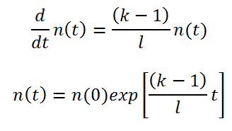
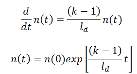
Finally, the change in the number of neutrons during a unit time interval dt is:
where:
n(t) = transient reactor power
n(0) = initial reactor power
τe = reactor period
The reactor period, τe, or e-folding time, is defined as the time required for the neutron density to change by a factor e = 2.718. The reactor period is usually expressed in units of seconds or minutes. The smaller the value of τe, the more rapid the change in reactor power. The reactor period may be positive or negative.
If there are neutrons in the system at t=0, that is, if n(0) > 0, the solution of this equation gives the simplest form of point kinetics equation (without source and delayed neutrons).
This simple point kinetics equation is often expressed in terms of reactivity and prompt generation time, Λ, as:
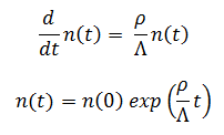
where
- ρ = (k-1)/k is the reactivity, which describes the deviation of an effective multiplication factor from unity.
- Λ = l/keff = prompt neutron generation time, the average time from a prompt neutron emission to absorption that results only in fission.
Both forms of the point kinetics equation are valid. The equation using Λ, prompt neutron generation time, is usually better for calculations. This is because most reactivity transients are induced by changes in the absorption cross-section rather than in the fission cross-section. The prompt neutron lifetime is not constant during these transients, whereas the prompt generation time remains constant.
Example:
Let us consider that the prompt neutron lifetime is ~2 x 10⁻⁵, and k (k∞ – neutron multiplication factor) will be step increased by only 0.01% (i.e., 10pcm or ~1.5 cents), that is, k∞=1.0000 will increase to k∞=1.0001.
It must be noted such reactivity insertion (10pcm) is very small in case of LWRs. The reactivity insertions of the order of one pcm are for LWRs practically unrealizable. In this case the reactor period will be:
T = l / (k∞ – 1) = 2 x 10⁻⁵ / (1.0001 – 1) = 0.2s
This is a very short period. In one second, the neutron flux (and power) in the reactor would increase by a factor of e5 = 2.7185. In 10 seconds, the reactor would pass through 50 periods, and the power would increase by e50.
Furthermore, in the case of fast reactors in which prompt neutron lifetimes are of the order of 10-7 seconds, the response of such a small reactivity insertion will be even more unimaginable. In the case of 10-7, the period will be:
T = l / (k∞ – 1) = 10-7 / (1.0001 – 1) = 0.001s
Reactors with such kinetics would be very difficult to control. Fortunately, this behavior is not observed in any multiplying system. Actual reactor periods are observed to be considerably longer than computed above, and therefore the nuclear chain reaction can be controlled more easily. The longer periods are observed due to the presence of the delayed neutrons.
ld = (1 – β).lp + ∑li . βi => ld = (1 – β).lp + ∑τi . βi
where
- (1 – β) is the fraction of all neutrons emitted as prompt neutrons
- lp is the prompt neutron lifetime
- τi is the mean precursor lifetime, the inverse value of the decay constant τi = 1/λi
- The weighted delayed generation time is given by τ = ∑τi . βi / β = 13.05 s
- Therefore the weighted decay constant λ = 1 / τ ≈ 0.08 s-1
The number, 0.08 s-1, is relatively high and has a dominating effect on reactor time response, although delayed neutrons are a small fraction of all neutrons in the core. This is best illustrated by calculating a weighted mean generation time with delayed neutrons:
ld = (1 – β).lp + ∑τi . βi = (1 – 0.0065). 2 x 10⁻⁵ + 0.085 = 0.00001987 + 0.085 ≈ 0.085
In short, the mean generation time with delayed neutrons is about ~0.1 s, rather than ~10-5 as in section Prompt Neutron Lifetime, where the delayed neutrons were omitted.
The role of ld is evident, and longer lifetimes give simply slower responses to multiplying systems. The role of reactivity (keff – 1) is also evident, and higher reactivity gives the simply larger response of the multiplying system.
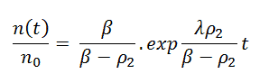
If there are neutrons in the system at t=0, that is, if n(0) > 0, the solution of this equation gives the simplest point kinetics equation with delayed neutrons (similarly to the case without delayed neutrons):
Example:
Let us consider that the mean generation time with delayed neutrons is ~0.085, and k (k∞ – neutron multiplication factor) will be step increased by only 0.01% (i.e., 10pcm or ~1.5 cents). That is, k∞=1.0000 will increase to k∞=1.0001.
It must be noted such reactivity insertion (10pcm) is very small in the case of LWRs (e.g., one step by control rods). The reactivity insertions of the order of one pcm are for LWRs practically unrealizable. In this case, the reactor period will be:
T = ld / (k∞-1) = 0.085 / (1.0001-1) = 850s
This is a very long period. In ~14 minutes, the neutron flux (and power) in the reactor would increase by a factor of e = 2.718. This is a completely different dimension of the response on reactivity insertion in comparison with the case without the presence of delayed neutrons, where the reactor period was 1 second.
Both simple point kinetics equations are only an approximation because they use many simplifications. The simple point kinetics equation with delayed neutrons completely fails for higher reactivity insertions, where is a significant difference between the production of prompt and delayed neutrons. Therefore a more accurate model is required. The exact point kinetics equations that can be derived from the general neutron balance equations without making any approximations are:
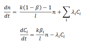
In the equation for neutrons, the first term on the right-hand side is the production of prompt neutrons in the present generation, k(1-β)n/l, minus the total number of neutrons in the preceding generation, -n/l. The second term is the production of delayed neutrons in the present generation. As can be seen, the rate of absorption of neutrons is the same as in the simple model (-n/l). But a distinction is between the direct channel for prompt neutrons (1-β) production and the delayed channel resulting from radioactive decay of precursor nuclei (λiCi).
In the equation for precursors, there is a balance between the production of the precursors of the i-th group and their decay after the decay constant λi. As can be seen, the decay rate of precursors is the radioactivity rate (λiCi). The production rate is proportional to the number of neutrons times βi, which is defined as the fraction of the neutrons that appear as delayed neutrons in the ith group.
As can be seen, the point kinetics equations include two differential equations, one for the neutron density n(t) and the other for precursors concentration C(t).
Again, the point kinetics equations are often expressed in terms of reactivity (ρ = (k-1)/k) and prompt generation time, Λ, as:
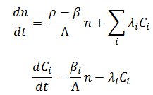
Both forms of the point kinetics equation are valid. The equation using Λ, prompt neutron generation time, is usually better for calculations. This is because most reactivity transients are induced by changes in the absorption cross-section rather than in the fission cross-section. The prompt neutron lifetime is not constant during these transients, whereas the prompt generation time remains constant.
The previous equation defines the reactivity of a reactor, which describes the deviation of an effective multiplication factor from unity. For critical conditions, the reactivity is equal to zero. The larger the absolute value of reactivity in the reactor core, the further the reactor is from criticality. The reactivity may be used to measure a reactor’s relative departure from criticality. According to the reactivity, we can classify the different reactor states and the related consequences as follows:
Approximate Solution of Point Kinetics Equations
Sometimes, it is convenient to predict qualitatively the behavior of a reactor. The exact solution can be obtained relatively easily using computers. Especially for illustration, the following approximations are discussed in the following sections:
- Prompt Jump Approximation
- Prompt Jump Approximation with One Group of Delayed Neutrons
- Constant Delayed Neutron Source Approximation
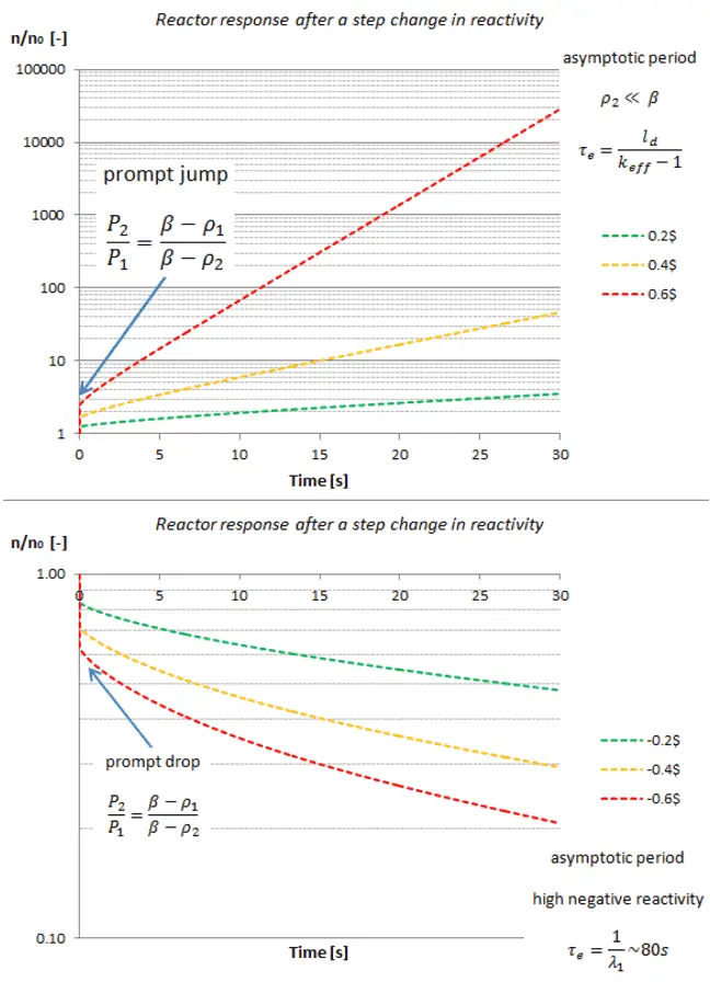
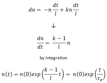
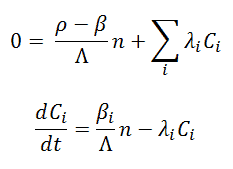
Suppose we are interested in long-term behavior (asymptotic period) and not interested in the details of the prompt jump. In that case, we can simplify the point kinetics equations by assuming that the prompt jump takes place instantaneously in response to any reactivity change. This approximation is known as the Prompt Jump Approximation (PJA). Due to prompt neutrons, the rapid power change is neglected, corresponding to taking dn/dt |0 = 0 in the point kinetics equations. That means the point kinetics equations are as follows:
From the equation for neutron flux and the assumption that the delayed neutron precursor population does not respond instantaneously to a change in reactivity (i.e., Ci,1 = Ci,2), it can be derived that the ratio of the neutron population just after and before the reactivity change is equal to:
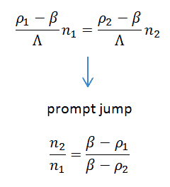
The prompt-jump approximation is usually valid for smaller reactivity insertion, for example, for ρ < 0.5β. It is usually used with another simplification and delayed precursor group approximation.
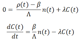
This simplification then leads to:
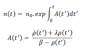
Assuming that the reactivity is constant and n1/n0 can be determined from the prompt jump formula, this equation leads to a very simple formula:
Suppose we are interested in short-term behavior and not interested in the details of the asymptotic behavior. In that case, we can simplify the point kinetics equations by assuming that the production of the delayed neutrons is constant and equal to the production at the beginning of the transient. This approximation is known as the Constant Delayed Neutron Source Approximation (CDS), in which changes in the number of delayed neutrons are neglected, corresponding to taking dCi(t)/dt = 0 and Ci(t) = Ci,0 in the point kinetics equations. That means the point kinetics equations are as follows:

The above equation can be solved analytically, and assuming that the reactivity is constant, the solution is given as:

Point Kinetics Equations – Notes
- the material composition of the system
- multiplying – non-multiplying system
- the system with or without thermalization
- isotopic composition of the system
- the geometric configuration of the system
- homogeneous or heterogeneous system
- the shape of the entire system
- size of the system
In an infinite reactor (without escape), prompt neutron lifetime is the sum of the slowing downtime and the diffusion time.
l=ts + td
In an infinite thermal reactor ts << td and therefore l ≈ td. The typical prompt neutron lifetime in thermal reactors is on the order of 10−4 seconds. Generally, the longer neutron lifetimes occur in systems in which the neutrons must be thermalized to be absorbed.
Most neutrons are absorbed in higher energies, and the neutron thermalization is suppressed (e.g., in fast reactors), having much shorter prompt neutron lifetimes. The typical prompt neutron lifetime in fast reactors is on the order of 10−7 seconds.

Source: Robert Reed Burn, Introduction to Nuclear Reactor Operation, 1988.
In multiplying systems, the absorption of a prompt fission neutron can initiate a fission reaction, l is equal to the average time between two generations of prompt neutrons (at keff=1). This time is known as the prompt neutron generation time.
Prompt Neutron Generation Time (or Mean Generation Time), Λ, is the average time from a prompt neutron emission to a capture that results only in fission. The prompt neutron generation time is designated as:
Λ = l/keff
The prompt generation time changes with the fuel burnup in power reactors, and in LWRs increases with the fuel burnup. It is simple, and fresh uranium fuel contains much fissile material (in the case of uranium fuel, about 4% of 235U). This causes significant excess of reactivity, and this excess must be compensated via chemical shim (in case of PWRs) or burnable absorbers.
The prompt neutron lives much shorter, and the prompt neutron lifetime is low due to these factors (high probability of absorption in fuel and high probability of absorption in moderator). With fuel burnup, the amount of fissile material as well as the absorption in moderator decreases, and therefore, the prompt neutron can “live” much longer.
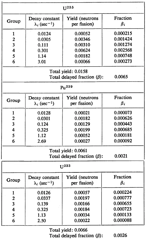
Reactor-kinetic calculations considering many initial conditions would be correct, but they would also be very complicated. Therefore G. R. Keepin and his co-workers suggested to group together the precursors based on their half-lives. Therefore delayed neutrons are traditionally represented by six delayed neutron groups, whose yields and decay constants (λ) are obtained from nonlinear least-squares fits experimental measurements. This model has the following disadvantages:
- All constants for each group of precursors are empirical fits to the data.
- They cannot be matched with decay constants of specific precursors.
- These constants are different for each fissionable nuclide.
- These constants also change with the neutron energy spectrum.
Although this six-group parameterization still satisfies the requirements of commercial organizations, higher accuracy of the delayed neutron yields and a better energy resolution in the delayed neutron spectra is desired.
It was recognized that the half-lives in the six-group structure do not accurately reproduce the asymptotic die-away time constants associated with the three longest-lived dominant precursors: 87Br, 137I, and 88Br.
This model may be insufficient, especially in the case of epithermal reactors, because virtually all delayed neutron activity measurements have been performed for fast or thermal-neutron-induced fission. In the case of fast reactors, the nuclear fission of six fissionable isotopes of uranium and plutonium is important, and the accuracy and energy resolution may play an important role.
A high-energy photon (gamma-ray) can, under certain conditions, eject a neutron from a nucleus. It occurs when its energy exceeds the binding energy of the neutron in the nucleus. Most nuclei have binding energies above 6 MeV, above the energy of most gamma rays from fission. On the other hand, few nuclei with sufficiently low binding energy are of practical interest. These are: 2D, 9Be, 6Li, 7Li, and 13C. As can be seen from the table, the lowest threshold have 9Be with 1.666 MeV and 2D with 2.226 MeV.
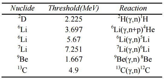
threshold energies.
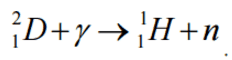
In the case of deuterium, neutrons can be produced by the interaction of gamma rays (with a minimum energy of 2.22 MeV) with deuterium:
Because gamma rays can be emitted by fission products with certain delays, and the process is very similar to that through which a “true” delayed neutron is emitted, photoneutrons are usually treated no differently than regular delayed neutrons in the kinetic calculations. Photoneutron precursors can also be grouped by their decay constant, similarly to “real” precursors. The table below shows the relative importance of source neutrons in CANDU reactors by showing the makeup of the full power flux.

Although photoneutrons are important, especially in CANDU reactors, deuterium nuclei are always present (~0.0156%) in the light water of LWRs. Moreover, the capture of neutrons in the hydrogen nucleus of the water molecules in the moderator yields small amounts of D2O, enhancing the heavy water concentration. Therefore, in LWRs kinetic calculations, photoneutrons from D2O are treated as additional groups of delayed neutrons with characteristic decay constants λj and effective group fractions.
After a nuclear reactor has been operating at full power for some time, there will be a considerable build-up of gamma rays from the fission products. This high gamma flux from short-lived fission products will decrease rapidly after shutdown. The photoneutron source decreases with the decay of long-lived fission products that produce delayed high-energy gamma rays in the long term. The photoneutron source drops slowly, decreasing a little each day. The longest-lived fission product with gamma-ray energy above the threshold is 140Ba with a half-life of 12.75 days.
The amount of fission products present in the fuel elements depends on how long the reactor has been operated before shutdown and at which power level has been the reactor operated before shutdown. Photoneutrons are usually a major source in a reactor and ensure sufficient neutron flux on source range detectors when the reactor is subcritical in long-term shutdown.
Compared with fission neutrons, which make a self-sustaining chain reaction possible, delayed neutrons make reactor control possible, and photoneutrons are important at low power operation.
See also: Effective Delayed Neutron Fraction – βeff
The delayed neutron fraction, β, is the fraction of delayed neutrons in the core at creation, that is, at high energies. But in the case of thermal reactors, the fission can be initiated mainly by a thermal neutron. Thermal neutrons are of practical interest in the study of thermal reactor behavior. The effective delayed neutron fraction usually referred to as βeff, is the same fraction at thermal energies.
The effective delayed neutron fraction reflects the ability of the reactor to thermalize and utilize each neutron produced. The β is not the same as the βeff due to the fact delayed neutrons do not have the same properties as prompt neutrons released directly from fission. In general, delayed neutrons have lower energies than prompt neutrons. Prompt neutrons have initial energy between 1 MeV and 10 MeV, with an average energy of 2 MeV. Delayed neutrons have initial energy between 0.3 and 0.9 MeV with an average energy of 0.4 MeV.
Therefore, a delayed neutron traverses a smaller energy range in thermal reactors to become thermal. It is also less likely to be lost by leakage or parasitic absorption than the 2 MeV prompt neutron. On the other hand, delayed neutrons are also less likely to cause fast fission because their average energy is less than the minimum required for fast fission to occur.
These two effects (lower fast fission factor and higher fast non-leakage probability for delayed neutrons) tend to counteract each other and form a term called the importance factor (I). The importance factor relates the average delayed neutron fraction to the effective delayed neutron fraction. As a result, the effective delayed neutron fraction is the product of the average delayed neutron fraction and the importance factor.
βeff = β . I
The delayed and prompt neutrons have a difference in their effectiveness in producing a subsequent fission event. Since the energy distribution of the delayed neutrons also differs from group to group, the different groups of delayed neutrons will also have different effectiveness. Moreover, a nuclear reactor contains a mixture of fissionable isotopes. Therefore, the importance factor is insufficient in some cases, and an importance function must be defined.
For example:
In a small thermal reactor with highly enriched fuel, the increase in fast non-leakage probability will dominate the decrease in the fast fission factor, and the importance factor will be greater than one.
In a large thermal reactor with low enriched fuel, the decrease in the fast fission factor will dominate the increase in the fast non-leakage probability, and the importance factor will be less than one (about 0.97 for a commercial PWR).
In large fast reactors, the decrease in the fast fission factor will also dominate the increase in the fast non-leakage probability, and the βeff is less than β by about 10%.
