Article Summary & FAQs
What is minor head loss?
In fluid flow, minor head loss or local loss is the loss of pressure or “head” in pipe flow due to the components as bends, fittings, valves, or heated channels.
Key Facts
- Head loss of the hydraulic system is divided into two main categories:
- Major Head Loss – due to friction in straight pipes
- Minor Head Loss – due to components as valves, bends…
- Minor head losses are a function of:
- flow regime (i.e., Reynolds number)
- flow velocity
- the geometry of a given component
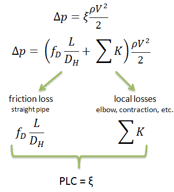
- Sometimes, engineers use the pressure loss coefficient, PLC. It is noted K or ξ (pronounced “xi”). This coefficient characterizes pressure loss of a certain hydraulic system or a part of a hydraulic system.
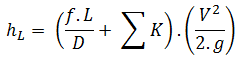
- A special form of Darcy’s equation can be used to calculate minor losses.
- The minor losses are roughly proportional to the square of the flow rate, and therefore they can be easily integrated into the Darcy-Weisbach equation through resistance coefficient K.
- As a local pressure loss, fluid acceleration in a heated channel can also be considered.
There are following methods:
- Equivalent length method
- K-method (resistance coeff. method)
- 2K-method
- 3K-method
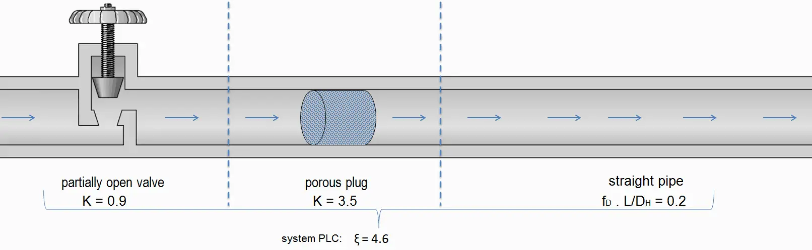
Sometimes, engineers use the pressure loss coefficient, PLC. It is noted K or ξ (pronounced “xi”). This coefficient characterizes pressure loss of a certain hydraulic system or a part of a hydraulic system. It can be easily measured in hydraulic loops. The pressure loss coefficient can be defined or measured for both straight pipes and especially for local (minor) losses.
Minor Head Loss – Local Losses
Any piping system contains different technological elements in the industry, such as bends, fittings, valves, or heated channels. These additional components add to the overall head loss of the system. Such losses are generally termed minor losses, although they often account for a major portion of the head loss. For relatively short pipe systems, with a relatively large number of bends and fittings, minor losses can easily exceed major losses (especially with a partially closed valve that can cause a greater pressure loss than a long pipe when a valve is closed or nearly closed, the minor loss is infinite).
The minor losses are commonly measured experimentally. The data, especially for valves, are somewhat dependent upon the particular manufacturer’s design.
Like pipe friction, the minor losses are roughly proportional to the square of the flow rate, and therefore they can be easily integrated into the Darcy-Weisbach equation. K is the sum of all of the loss coefficients in the length of pipe, each contributing to the overall head loss.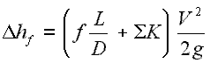
There are several methods how to calculate head loss from fittings, bends, and elbows. In the following section, these methods are summarized from the simplest to the most sophisticated.
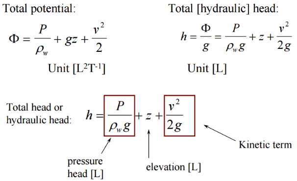
In fluid dynamics, the head is a concept that relates the energy in an incompressible fluid to the height of an equivalent static column of that fluid. The units for all the different forms of energy in Bernoulli’s equation can also be measured in distance units. Therefore these terms are sometimes referred to as “heads” (pressure head, velocity head, and elevation head). Head is also defined for pumps. This head is usually referred to as the static head and represents the maximum height (pressure) it can deliver. Therefore the characteristics of all pumps can usually be read from their Q-H curve (flow rate – height).
There are four types of potential (head):
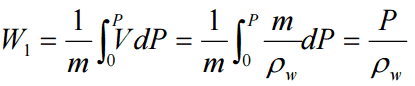
- Pressure potential – Pressure head: The pressure head represents the flow energy of a column of fluid whose weight is equivalent to the pressure of the fluid.
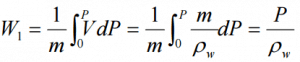 ρw: density of water assumed to be independent of pressure
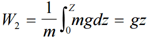
 - Elevation potential – Elevation head: The elevation head represents the potential energy of a fluid due to its elevation above a reference level.
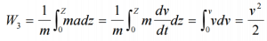
- Kinetic potential – Kinetic head: The kinetic head represents the kinetic energy of the fluid. The height in feet is that a flowing fluid would rise in a column if all of its kinetic energy were converted to potential energy.

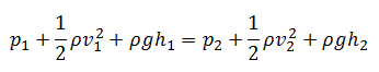
The sum of a fluid’s elevation head, kinetic head, and pressure head is called the total head. Thus, Bernoulli’s equation states that the total head of the fluid is constant.
Consider a pipe containing an ideal fluid. Suppose this pipe undergoes a gradual expansion in diameter. In that case, the continuity equation tells us that as the pipe diameter increases, the flow velocity must decrease to maintain the same mass flow rate. Since the outlet velocity is less than the inlet velocity, the kinetic head of the flow must decrease from the inlet to the outlet. If there is no change in the elevation head (the pipe lies horizontally), the decrease in the kinetic head must be compensated for by an increase in pressure head.
Equivalent Length Method
The equivalent length method (The Le/D method) allows the user to describe the pressure loss through an elbow or a fitting as a length of straight pipe.
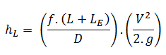
This method is based on the observation that the major losses are also proportional to the velocity head (v2/2g).

The Le/D method increases the multiplying factor in the Darcy-Weisbach equation (i.e., ƒ.L/D) by a length of straight pipe (i.e., Le) which would give rise to a pressure loss equivalent to the losses in the fittings, hence the name “equivalent length”. The multiplying factor, therefore, becomes ƒ(L+Le)/D and the equation for calculation of pressure loss of the system is, therefore:
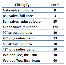 All fittings, elbows, tees can be summed up to make one total length, and the pressure loss is calculated from this length. It has been experimentally found that if the equivalent lengths for a range of sizes of a given type of fitting are divided by the diameters of the fittings, then an almost constant ratio (i.e., Le/D) is obtained. The advantage of the equivalent length method is that a single data value is sufficient to cover all sizes of that fitting. Therefore the tabulation of equivalent length data is relatively easy. Some typical equivalent lengths are shown in the table.
See also: Pipe Sizing and Flow Calculation Software
Resistance Coefficient Method – K Method – Excess head
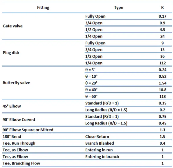 The resistance coefficient method (or K-method, or Excess head method) allows the user to describe the pressure loss through an elbow or a fitting by a dimensionless number – K. This dimensionless number (K) can be incorporated into the Darcy-Weisbach equation in a very similar way to the equivalent length method. Instead of equivalent length data, in this case, the dimensionless number (K) is used to characterize the fitting without linking it to the properties of the pipe.
The K-value represents the multiple velocity heads that the fluid passing will lose through the fitting. The equation for calculation of pressure loss of the hydraulic element is, therefore:
 Therefore the equation for calculation of pressure loss of the entire hydraulic system is:
The K-value can be characterized for various flow regimes (i.e., according to the Reynolds number), and this causes it to be more accurate than the equivalent length method.
There are several other methods for calculating pressure loss for fittings, and these methods are more sophisticated and also more accurate:
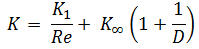
- 2K-Method. The 2K method is a technique developed by Hooper B.W. to predict head loss in an elbow, valve, or tee. The 2K method improves the excess head method by characterizing the change in pressure loss due to varying Reynolds number. The 2-K method is advantageous over other methods, especially in the laminar flow region.
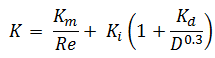
- 3K-Method. The 3K method (by Ron Darby in 1999) further improves the accuracy of the pressure loss calculation by also characterizing the change in geometric proportions of a fitting as its size changes. This makes the 3K method particularly accurate for a system with large fittings.

Flow-through Elbow – Minor Loss
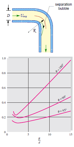 The flow-through elbows are quite complicated. Any curved pipe always induces a larger loss than the simple straight pipe. This is because, in a curved pipe, the flow separates on the curved walls. For a very small radius of curvature, the incoming flow is unable to make the turn at the bend. Therefore the flow separates and in part stagnates against the opposite side of the pipe. In this part of the bend, the pressure raises (as a result of Bernoulli’s principle), and the velocity decreases.
An interesting feature of the K-values for elbows is their non-monotone behavior as the R/D ratio increases. The K-values include both the local losses and frictional losses of the pipe. The local losses, caused by flow separation and secondary flow, decrease with R/D, while the frictional losses increase because the bend length increases. Therefore there is a minimum in the K-value near the normalized radius of curvature of 3.
Fluid Acceleration
It is known that when the fluid is heated (e.g.,, in a fuel channel), the fluid expands (change in the fluid density) and increases its flow velocity as a result of the continuity equation (the channel cross-section remains the same). For a control volume that has a single inlet and a single outlet, this equation states that, for steady-state flow, the mass flow rate into the volume must equal the mass flow rate out.
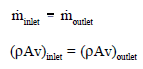
Mass entering per unit time = mass leaving per unit time
See also: Subcooled Water Properties
Another very important principle states (Bernoulli’s principle) that the increase in flow velocity in the heated channel causes the lowering of fluid pressure. This pressure loss can also be considered as a local pressure loss and can be calculated from the following equation:
![]()
The flow rate through a reactor core – coolant acceleration
It is an illustrative example, and the following data do not correspond to any reactor design.

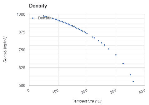
Pressurized water reactors are cooled and moderated by high-pressure liquid water (e.g.,, 16MPa). At this pressure, water boils at approximately 350°C (662°F). The inlet temperature of the water is about 290°C (⍴ ~ 720 kg/m3). The water (coolant) is heated in the reactor core to approximately 325°C (⍴ ~ 654 kg/m3) as the water flows through the core.
The primary circuit of typical PWRs is divided into 4 independent loops (piping diameter ~ 700mm). Each loop comprises a steam generator and one main coolant pump. Inside the reactor pressure vessel (RPV), the coolant first flows down outside the reactor core (through the downcomer). The flow is reversed up through the core from the bottom of the pressure vessel, where the coolant temperature increases as it passes through the fuel rods and the assemblies formed by them.
Calculate:
- Pressure loss due to the coolant acceleration in an isolated fuel channel
when
- channel inlet flow velocity is equal to 5.17 m/s
- channel outlet flow velocity is equal to 5.69 m/s
Solution:
The pressure loss due to the coolant acceleration in an isolated fuel channel is then:

This fact has important consequences. Due to the different relative power of fuel assemblies in a core, these fuel assemblies have different hydraulic resistance. This may induce a local lateral flow of primary coolant and must be considered in thermal-hydraulic calculations.