General Form
Using these two equations, we can derive the general heat conduction equation:

This equation is also known as the Fourier-Biot equation and provides the basic tool for heat conduction analysis.
In previous sections, we have dealt with one-dimensional steady-state heat transfer, which can be characterized by Fourier’s law of heat conduction. But its applicability is very limited. This law assumes steady-state heat transfer through a planar body (note that Fourier’s law can also be derived for cylindrical and spherical coordinates) without heat sources. The rate equation is in this heat transfer mode, where the temperature gradient is known.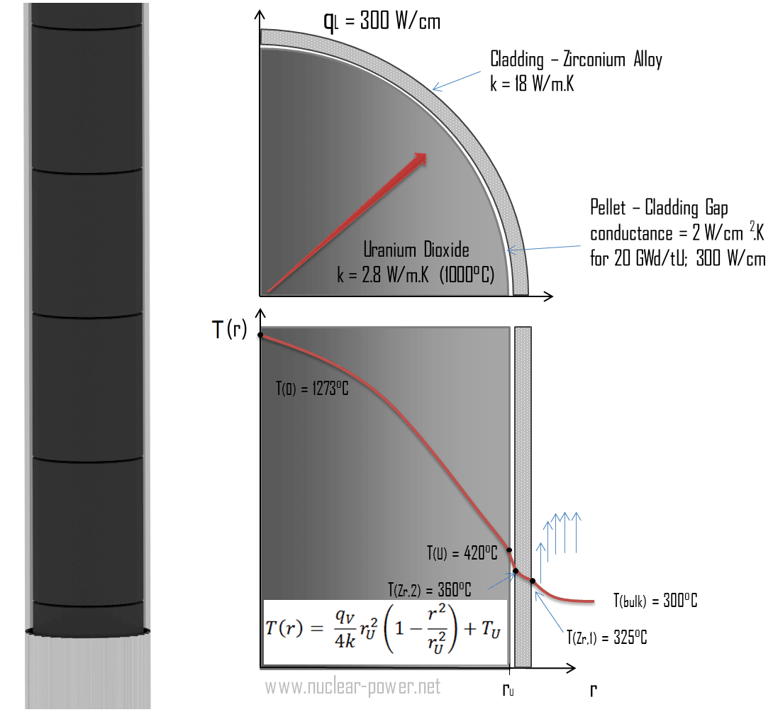
But a major problem in most conduction analyses is determining the temperature field in a medium resulting from conditions imposed on its boundaries. In engineering, we have to solve heat transfer problems involving different geometries and different conditions, such as a cylindrical nuclear fuel element, which involves an internal heat source or the wall of a spherical containment. These problems are more complex than the planar analyses in previous sections. Therefore these problems will be the subject of this section, in which the heat conduction equation will be introduced and solved.
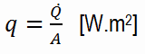
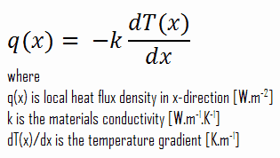
where A is the heat transfer area. The unit of heat flux in English units is Btu/h·ft2. Note that heat flux may vary with time and position on a surface.
In nuclear reactors, limitations of the local heat flux are of the highest importance for reactor safety. Since nuclear fuel consists of fuel rods, the heat flux is defined in units of W/cm (local linear heat flux) or kW/rod (power per fuel rod).
General Heat Conduction Equation
The heat conduction equation is a partial differential equation that describes heat distribution (or the temperature field) in a given body over time. Detailed knowledge of the temperature field is very important in thermal conduction through materials. Once this temperature distribution is known, the conduction heat flux at any point in the material or on its surface may be computed from Fourier’s law.
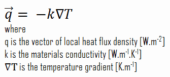
The heat equation is derived from Fourier’s law and conservation of energy. Fourier’s law states that the time rate of heat transfer through a material is proportional to the negative gradient in the temperature and the area at right angles to that gradient through which the heat flows.
A change in internal energy per unit volume in the material, ΔQ, is proportional to the change in temperature, Δu. That is:
∆Q = ρ.cp.∆T
General Form
Using these two equations, we can derive the general heat conduction equation:
This equation is also known as the Fourier-Biot equation and provides the basic tool for heat conduction analysis. From its solution, we can obtain the temperature field as a function of time.
In words, the heat conduction equation states that:
At any point in the medium, the net rate of energy transfer by conduction into a unit volume plus the volumetric rate of thermal energy generation must equal the rate of change of thermal energy stored within the volume.
The thermal conductivity of most liquids and solids varies with temperature, and for vapors, it also depends upon pressure. In general:
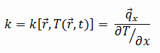
Most materials are nearly homogeneous. Therefore, we can usually write k = k (T). Similar definitions are associated with thermal conductivities in the y- and z-directions (ky, kz), but for an isotropic material, the thermal conductivity is independent of the direction of transfer, kx = ky = kz = k.
The previous equation follows that the conduction heat flux increases with increasing thermal conductivity and increasing temperature differences. In general, the thermal conductivity of a solid is larger than that of a liquid, which is larger than that of a gas. This trend is due largely to differences in intermolecular spacing for the two states of matter. In particular, diamond has the highest hardness and thermal conductivity of any bulk material.
See also: Thermal Conductivity
 Most of PWRs use uranium fuel, which is in the form of uranium dioxide. Uranium dioxide is a black semiconducting solid with very low thermal conductivity. On the other hand, uranium dioxide has a very high melting point and has well-known behavior. The UO2 is pressed into pellets, and these pellets are then sintered into the solid.
These pellets are then loaded and encapsulated within a fuel rod (or fuel pin) made of zirconium alloys due to their very low absorption cross-section (unlike stainless steel). The surface of the tube, which covers the pellets, is called fuel cladding. Fuel rods are the base element of a fuel assembly.
The thermal conductivity of uranium dioxide is very low compared with metal uranium, uranium nitride, uranium carbide, and zirconium cladding material. Thermal conductivity is one of the parameters which determine the fuel centerline temperature. This low thermal conductivity can result in localized overheating in the fuel centerline, and therefore this overheating must be avoided. Overheating of the fuel is prevented by maintaining the steady-state peak linear heat rate (LHR) or the Heat Flux Hot Channel Factor – FQ(z) below the level at which fuel centerline melting occurs. Expansion of the fuel pellet upon centerline melting may cause the pellet to stress the cladding to the point of failure.
Thermal conductivity of solid UO2 with a density of 95% is estimated by the following correlation [Klimenko; Zorin]:
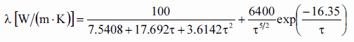
where τ = T/1000. The uncertainty of this correlation is +10% in the range from 298.15 to 2000 K and +20% in the range from 2000 to 3120 K.

Special reference: Thermal and Nuclear Power Plants/Handbook ed. by A.V. Klimenko and V.M. Zorin. MEI Press, 2003.
Special reference: Thermophysical Properties of Materials For Nuclear Engineering: A Tutorial and Collection of Data. IAEA-THPH, IAEA, Vienna, 2008. ISBN 978–92–0–106508–7.
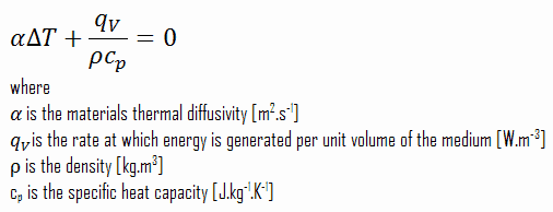
This equation can be further reduced assuming the thermal conductivity to be constant and introducing the thermal diffusivity, α = k/ρcp:
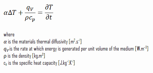
 In heat transfer analysis, the ratio of the thermal conductivity to the specific heat capacity at constant pressure is an important property termed the thermal diffusivity. The thermal diffusivity appears in the transient heat conduction analysis and the heat equation.
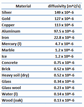
It represents how fast heat diffuses through the material and has units m2/s. In other words, it is the measure of the thermal inertia of given material. Thermal diffusivity is usually denoted α and is given by:
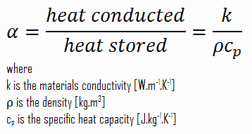
As can be seen, it measures the ability of a material to conduct thermal energy (represented by factor k) relative to its ability to store thermal energy (represented by factor ρ.cp). Materials of large α will respond quickly to changes in their thermal environment. In contrast, materials of small α will respond more slowly (heat is mostly absorbed), taking longer to reach a new equilibrium condition.
Additional simplifications of the general form of the heat equation are often possible. For example, under steady-state conditions, there can be no change in the amount of energy storage (∂T/∂t = 0).
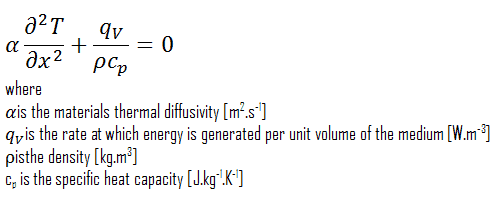
One-dimensional Heat Equation
One of the most powerful assumptions is the special case of one-dimensional heat transfer in the x-direction. In this case, the derivatives for y and z drop out, and the equations above reduce to (Cartesian coordinates):
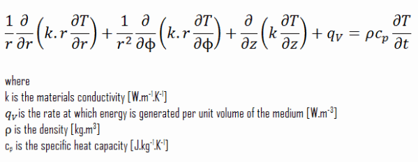
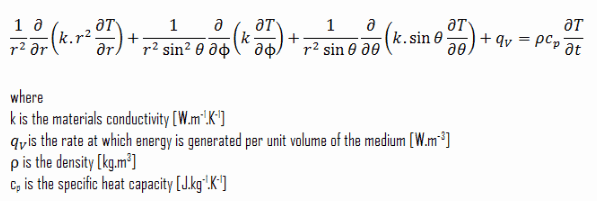
Heat Conduction in Cylindrical and Spherical Coordinates
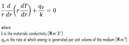
There are plenty of problems in engineering that cannot be solved in cartesian coordinates. Cylindrical and spherical systems are very common in thermal and power engineering, and the heat equation may also be expressed in cylindrical and spherical coordinates. The general heat conduction equation in cylindrical coordinates can be obtained from an energy balance on a volume element in cylindrical coordinates and using the Laplace operator, Δ, in the cylindrical and spherical form.
Cylindrical coordinates:
Spherical coordinates:
Obtaining analytical solutions to these differential equations requires a knowledge of the solution techniques of partial differential equations, which is beyond the scope of this text. On the other hand, there are many simplifications and assumptions that can be applied to these equations, leading to very important results. The next section limits our consideration to one-dimensional steady-state cases with constant thermal conductivity since they result in ordinary differential equations.
Boundary and Initial Conditions
As for another differential equation, the solution is given by boundary and initial conditions. Several common possibilities are simply expressed in the mathematical form concerning the boundary conditions.
Because the heat equation is second order in the spatial coordinates, two boundary conditions must be given for each direction of the coordinate system, along which heat transfer is significant to describe a heat transfer problem completely. Therefore, we need to specify four boundary conditions for two-dimensional problems and six boundary conditions for three-dimensional problems.
Four kinds of boundary conditions commonly encountered in heat transfer are summarized in the following section:
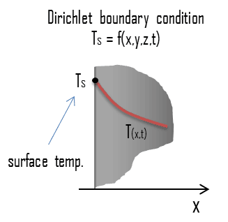 In mathematics, the Dirichlet (or first-type) boundary condition is a type of boundary condition, named after a German mathematician Peter Gustav Lejeune Dirichlet (1805–1859). When imposed on an ordinary or a partial differential equation, the condition specifies the values in which the derivative of a solution is applied within the domain’s boundary.
This condition corresponds to a given fixed surface temperature in heat transfer problems. The Dirichlet boundary condition is closely approximated, for example, when the surface is in contact with a melting solid or a boiling liquid. In both cases, there is heat transfer at the surface, while the surface remains at the temperature of the phase change process.
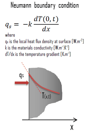 In mathematics, the Neumann (or second-type) boundary condition is a type of boundary condition, named after a German mathematician Carl Neumann (1832–1925). When imposed on an ordinary or a partial differential equation, it specifies the values that a solution needs to take along the domain’s boundary.
In heat transfer problems, the Neumann condition corresponds to a given rate of change of temperature. In other words, this condition assumes that the heat flux at the material’s surface is known. The heat flux in the positive x-direction anywhere in the medium, including the boundaries, can be expressed by Fourier’s law of heat conduction.
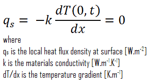
Special Case – Adiabatic Boundary – Perfectly Insulated Boundary
A special case of this condition corresponds to the perfectly insulated surface for which (∂T/∂x = 0). Heat transfer through a properly insulated surface can be zero since adequate insulation reduces heat transfer through a surface to negligible levels. Mathematically, this boundary condition can be expressed as:
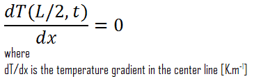
Special Case – Thermal Symmetry
 Another very important case that can be used for solving heat transfer problems involving fuel rods is thermal symmetry. For example, the two surfaces of a large hot plate of thickness L suspended vertically in the air will be subjected to the same thermal conditions. Thus, the temperature distribution will be symmetrical (i.e., one half of the plate will be the same temperature profile as the other half). As a result, there must be a maximum in the centerline of the plate, and the centerline can be viewed as an insulated surface (∂T/∂x = 0). The thermal condition at this plane of symmetry can be expressed as:
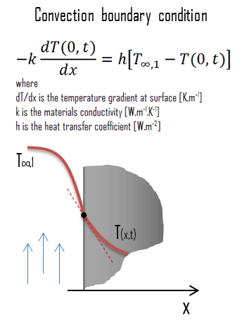 In heat transfer problems, the convection boundary condition, also known as the Newton boundary condition, corresponds to the existence of convection heating (or cooling) at the surface and is obtained from the surface energy balance. The convection boundary condition is probably the most common boundary condition encountered in practice since most heat transfer surfaces are exposed to a convective environment at specified parameters.
In other words, this condition assumes that the heat conduction at the material’s surface is equal to the heat convection at the surface in the same direction. Since the boundary cannot store energy, the net heat entering the surface from the convective side must leave the surface from the conduction side.
Similarly, the radiation boundary condition can be constructed and used.
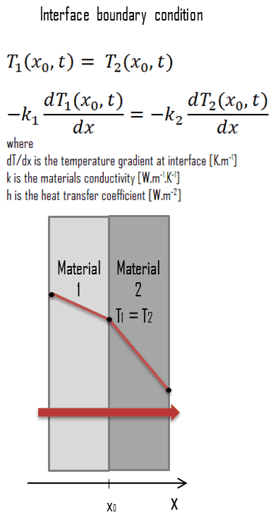 In heat transfer problems, the interface boundary condition can be used when the material is made up of layers of different materials. The solution of a heat transfer problem in such a medium requires the solution of the heat transfer problem in each layer, and one must specify an interface condition at each interface. The interface boundary conditions at an interface are based on the two following requirements:
- two bodies in contact must have the same temperature at the area of contact (i.e., an ideal contact without contact resistance)
- an interface cannot store any energy, and therefore the heat conduction at the surface of the first material is equal to the heat conduction at the surface of the second material
Noteworthy, when components are bolted or otherwise pressed together, a knowledge of the thermal performance of such joints is also needed. The temperature drop across the interface between materials may be appreciable in these composite systems. This temperature drop is characterized by the thermal contact conductance coefficient, hc, which indicates the thermal conductivity, or ability to conduct heat, between two bodies in contact.
The interface boundary condition can be mathematically expressed in the way depicted in the figure.
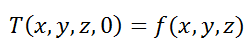
where the function f(x, y, z) represents the temperature field inside the material at time t = 0. Note that under steady conditions, the heat conduction equation does not involve any time derivatives (∂T/∂t = 0), and thus we do not need to specify an initial condition.
Conduction with Heat Generation
We considered thermal conduction problems without internal heat sources in the preceding section. For these problems, the temperature distribution in a medium was determined solely by conditions at the boundaries of the medium. But in engineering, we can often meet a problem in which internal heat sources are significant and determine the temperature distribution together with boundary conditions.
These problems are of the highest importance in nuclear engineering since most of the heat generated in nuclear fuel is released inside the fuel pellets. The temperature distribution is determined primarily by heat generation distribution. Note that, as can be seen from the description of the individual components of the total energy released during the fission reaction, there is a significant amount of energy generated outside the nuclear fuel (outside fuel rods). Especially the kinetic energy of prompt neutrons is largely generated in the coolant (moderator). This phenomenon needs to be included in the nuclear calculations.
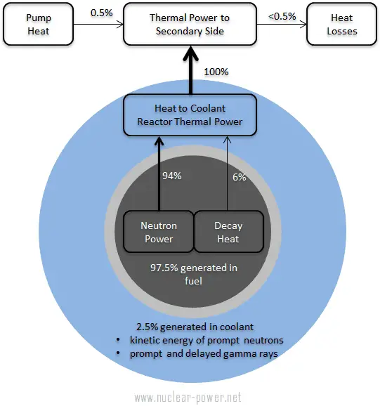
For LWR, it is generally accepted that about 2.5% of total energy is recovered in the moderator. This fraction of energy depends on the materials, their arrangement within the reactor, and thus on the reactor type.
Note that heat generation is a volumetric phenomenon. That is, it occurs throughout the body of a medium. Therefore, the heat generation rate in a medium is usually specified per unit volume and is denoted by gV [W/m3].
The temperature distribution and accordingly the heat flux is primarily determined by:
- Geometry and boundary conditions. Different geometry leads to completely different temperature fields.
- Heat generation rate. The temperature drop through the body will increase with increased heat generation.
- Thermal conductivity of the medium. Higher thermal conductivity will lead to lower temperature drop.
Solution of Heat Equation

The general solution of this equation is:
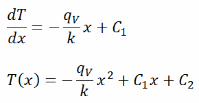
where C1 and C2 are the constants of integration.
1)
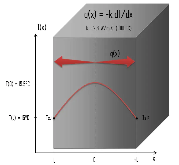 Calculate the temperature distribution, T(x), through this thick plane wall, if:
- the temperatures at both surfaces are 15.0°C
- the thickness of this wall is 2L = 10 mm.
- the material’s conductivity is k = 2.8 W/m.K (corresponds to uranium dioxide at 1000°C)
- the volumetric heat rate is qV = 106 W/m3
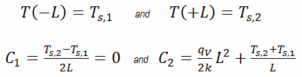
In this case, the surfaces are maintained at given temperatures Ts,1 and Ts,2. This corresponds to the Dirichlet boundary condition. Moreover, this problem is thermally symmetric, and therefore we may also use thermal symmetry boundary conditions. The constants may be evaluated using substitution into the general solution and are of the form:
The resulting temperature distribution and the centerline (x = 0) temperature (maximum) in this plane wall at these specific boundary conditions will be:
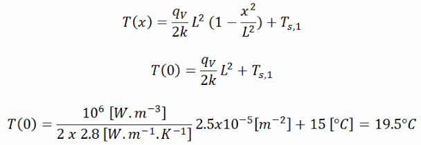
The heat flux at any point, qx [W.m-2], in the wall may, of course, be determined by using the temperature distribution and with Fourier’s law. Note that, with heat generation, the heat flux is no longer independent of x, the, therefore:
These cylindrical pellets are then loaded and encapsulated within a fuel rod (or fuel pin) made of zirconium alloys due to their very low absorption cross-section (unlike stainless steel). The surface of the tube, which covers the pellets, is called fuel cladding.
See also: Thermal Conduction of Uranium Dioxide
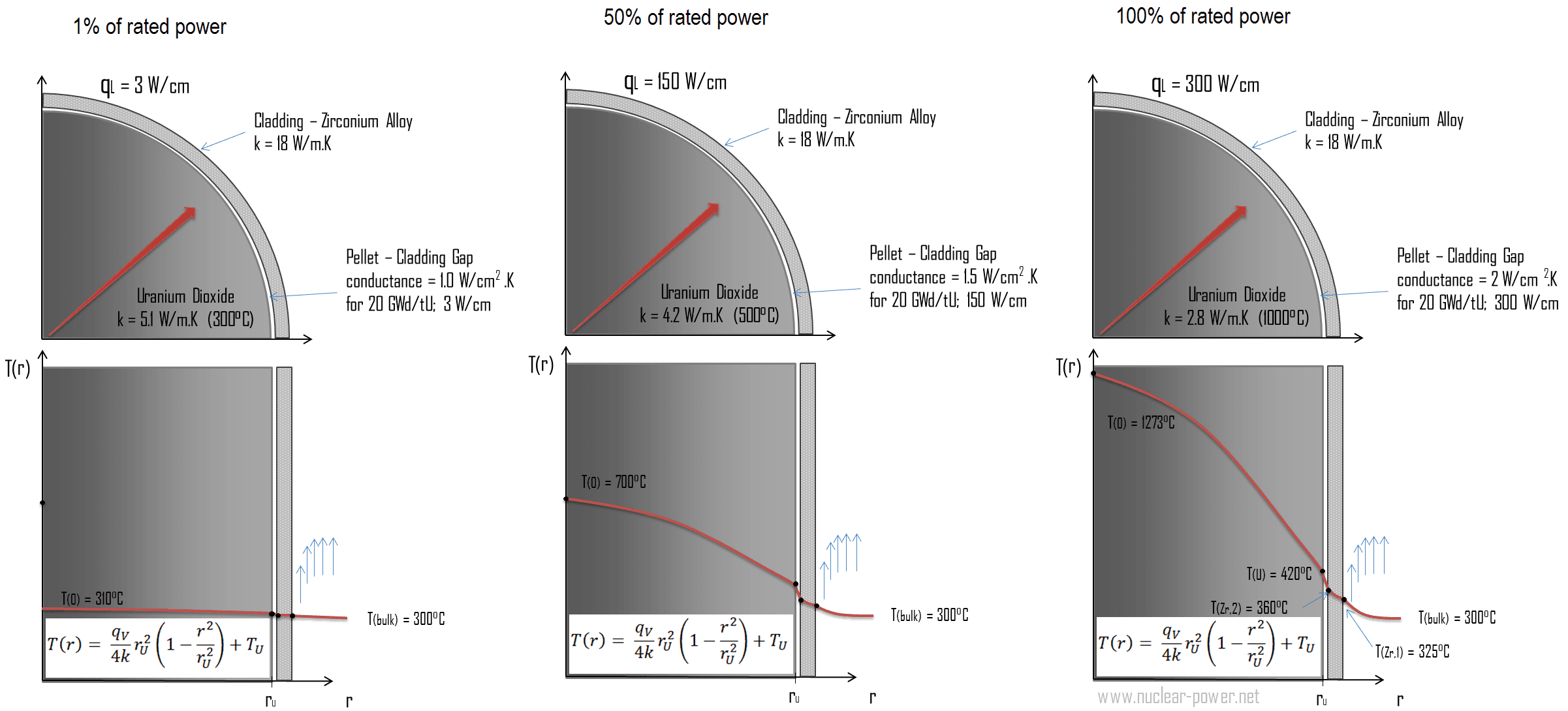
The thermal and mechanical behavior of fuel pellets and fuel rods constitute one of three key core design disciplines. Nuclear fuel is operated under inhospitable conditions (thermal, radiation, mechanical) and must withstand more than normal conditions operation. For example, temperatures in the center of fuel pellets reach more than 1000°C (1832°F), accompanied by fission-gas releases. Therefore detailed knowledge of temperature distribution within a single fuel rod is essential for the safe operation of nuclear fuel. This section will study the heat conduction equation in cylindrical coordinates using Dirichlet boundary conditions with given surface temperature (i.e., using Dirichlet boundary condition). Comprehensive analysis of fuel rod temperature profile will be studied separately.
The temperature in the centerline of a fuel pellet
Consider the fuel pellet of radius rU = 0.40 cm, in which there is uniform and constant heat generation per unit volume, qV [W/m3]. Instead of volumetric heat rate qV [W/m3], engineers often use the linear heat rate, qL [W/m], representing the heat rate of one meter of a fuel rod. The linear heat rate can be calculated from the volumetric heat rate by:
![]()
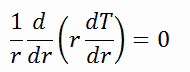
The centreline is taken as the origin for r-coordinate. Due to symmetry in the z-direction and azimuthal direction, we can separate variables and simplify this problem into one-dimensional. Thus, we will only solve for the temperature as a function of radius, T(r). For constant thermal conductivity, k, the appropriate form of the cylindrical heat equation, is:
The general solution of this equation is:
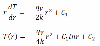
where C1 and C2 are the constants of integration.
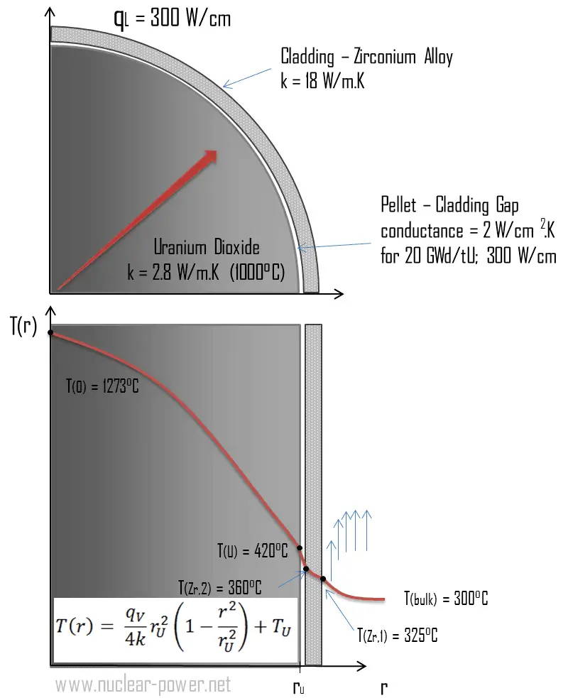 Calculate the temperature distribution, T(r), in this fuel pellet, if:
- the temperature at the surface of the fuel pellet is TU = 420°C
- the fuel pellet radius rU = 4 mm.
- the averaged material’s conductivity is k = 2.8 W/m.K (corresponds to uranium dioxide at 1000°C)
- the linear heat rate is qL = 300 W/cm and thus the volumetric heat rate is qV = 597 x 106 W/m3
In this case, the surface is maintained at given temperatures TU. This corresponds to the Dirichlet boundary condition. Moreover, this problem is thermally symmetric, and therefore we may also use thermal symmetry boundary conditions. The constants may be evaluated using substitution into the general solution and are of the form:
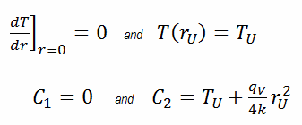
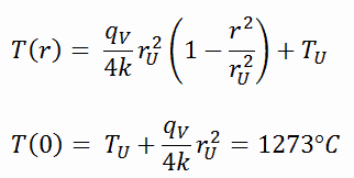
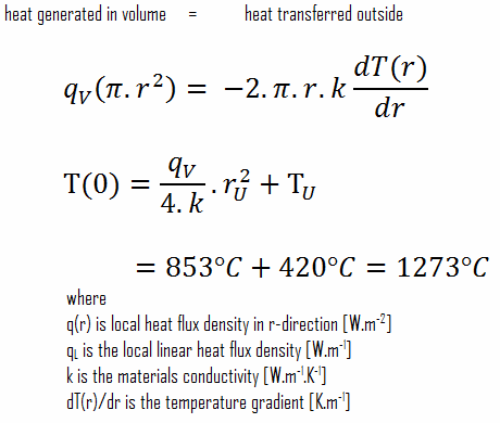
The resulting temperature distribution and the centerline (r = 0) temperature (maximum) in this cylindrical fuel pellet at these specific boundary conditions will be:
The radial heat flux at any radius, qr [W.m-1], in the cylinder may, of course, be determined by using the temperature distribution and with Fourier’s law. Note that, with heat generation, the heat flux is no longer independent of r.
∆T in fuel pellet
Detailed knowledge of geometry, the outer radius of fuel pellet, volumetric heat rate, and the pellet surface temperature (TU) determines ∆T between outer surface and centerline of fuel pellet. Therefore we can calculate the centerline temperature (TZr,2) simply using the energy conservation between heat generated in the volume and the transferred outside the volume:
The following figure shows the temperature distribution in the fuel pellet at various power levels.
______
The temperature in an operating reactor varies from point to point within the system. Consequently, there is always one fuel rod and one local volume hotter than all the rest. The peak power limits must be introduced to limit these hot places. The peak power limits are associated with a boiling crisis and conditions that could cause fuel pellet melt. However, metallurgical considerations place upper limits on the fuel cladding temperature and the fuel pellet. Above these temperatures, there is a danger that the fuel may be damaged. One of the major objectives in the design of nuclear reactors is to remove the heat produced at the desired power level while assuring that the maximum fuel temperature and the maximum cladding temperature are always below these predetermined values.
Consider the fuel cladding of inner radius rZr,2 = 0.408 cm and outer radius rZr,1 = 0.465 cm. Compared to fuel pellet, there is almost no heat generation in the fuel cladding (cladding is slightly heated by radiation). All heat generated in the fuel must be transferred via conduction through the cladding, and therefore, the inner surface is hotter than the outer surface.
To find the temperature distribution through the cladding, we must solve the heat conduction equation. Due to symmetry in the z-direction and the azimuthal direction, we can separate variables and simplify this problem to a one-dimensional problem. Thus, we will only solve for the temperature as a function of radius, T(r). In this example, we will assume that there is strictly no heat generation within the cladding. For constant thermal conductivity, k, the appropriate form of the cylindrical heat equation, is:
The general solution of this equation is:

where C1 and C2 are the constants of integration.
1)
Calculate the temperature distribution, T(r), in this fuel cladding, if:
- the temperature at the inner surface of the cladding is TZr,2 = 360°C
- the temperature of reactor coolant at this axial coordinate is Tbulk = 300°C
- the heat transfer coefficient (convection; turbulent flow) is h = 41 kW/m2.K.
- the averaged material’s conductivity is k = 18 W/m.K
- the linear heat rate of the fuel is qL = 300 W/cm, and thus, the volumetric heat rate is qV = 597 x 106 W/m3
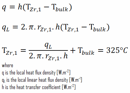
From the basic relationship for heat transfer by convection, we can calculate the outer surface of the cladding as:
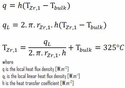
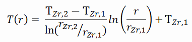
As can be seen, in this case, we have given surface temperatures TZr,1 and TZr,2. This corresponds to the Dirichlet boundary condition. The constants may be evaluated using substitution into the general solution and are of the form:

Solving for C1 and C2 and substituting into the general solution, we then obtain:
∆T – cladding surface – coolant
Detailed knowledge of geometry, the outer radius of cladding, linear heat rate, convective heat transfer coefficient, and the coolant temperature determines ∆T between the coolant (Tbulk) and the cladding surface (TZr,1). Therefore we can calculate the cladding surface temperature (TZr,1) simply using Newton’s Law:
∆T in fuel cladding
Detailed knowledge of geometry, outer and inner radius of cladding, linear heat rate, and the cladding surface temperature (TZr,1) determine ∆T between outer and inner surfaces of cladding. Therefore we can calculate the inner cladding surface temperature (TZr,2) simply using Fourier’s Law:
