In the practical analysis of piping systems, the quantity of most importance is the pressure loss due to viscous effects along the length of the system, as well as additional pressure losses arising from other technological equipments like valves, elbows, piping entrances, fittings, and tees.
In contrast, to single-phase pressure drops, calculation and prediction of two-phase pressure drops is a much more sophisticated problem, and leading methods differ significantly. Experimental data indicates that the frictional pressure drop in the two-phase flow (e.g.,, in a boiling channel) is substantially higher than for a single-phase flow with the same length and mass flow rate. Explanations include an increased surface roughness due to bubble formation on the heated surface and increased flow velocities.
Pressure Drop – Homogeneous Flow Model
The simplest approach to predicting two-phase flows is to treat the entire two-phase flow as if it were all liquid, except flowing at the two-phase mixture velocity. The two-phase pressure drops for flows inside pipes and channels are the sum of three contributions:
- the static pressure drop ∆pstatic (elevation head)
- the momentum pressure drop ∆pmom (fluid acceleration)
- the frictional pressure drop ∆pfrict
The total pressure drop of the two-phase flow is then:
∆ptotal = ∆pstatic + ∆pmom + ∆pfrict
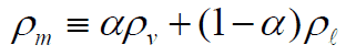
The static and momentum pressure drops can be calculated similarly as in the case of single-phase flow and using the homogeneous mixture density:
The most problematic term is the frictional pressure drop ∆pfrict, which is based on the single-phase pressure drop multiplied by the two-phase correction factor (homogeneous friction multiplier – Φlo2). By this approach, the frictional component of the two-phase pressure drop is:

where (dP/dz)2f is frictional pressure gradient of two-phase flow and (dP/dz)1f is frictional pressure gradient if an entire flow (of total mass flow rate G) flows like a liquid in the channel (standard single-phase pressure drop). The term Φlo2 is the homogeneous friction multiplier that can be derived according to various methods. One of the possible multipliers is equal to Φlo2 = (1+xg(ρl/ρg – 1)) and therefore:
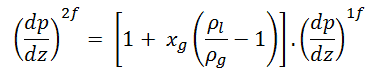
As can be seen, this simple model suggests that the two-phase frictional losses are in any event higher than the single-phase frictional losses. The homogeneous friction multiplier increases rapidly with flow quality.
Typical flow qualities in steam generators and BWR cores are on the order of 10 to 20 %. The corresponding two phase frictional loss would then be 2 – 4 times that in an equivalent single-phase system.
Source: http://authors.library.caltech.edu/25021/1/chap8.pdf
In this model, the phases are considered to be flowing separately in the channel, each occupying a given fraction of the channel cross-section and each with a given velocity. It is obvious the predicting the void fraction is very important for these methods. Numerous methods are available for predicting the void fraction.
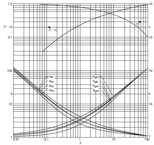
The method of Lockhart and Martinelli is the original method that predicted the two-phase frictional pressure drop based on a friction multiplicator for the liquid-phase or the vapor-phase:
∆pfrict = Φltt2 . ∆pl (liquid-phase ∆p)
∆pfrict = Φgtt2 . ∆pg (vapor-phase ∆p)
The single-phase friction factors of the liquid fl and the vapor fg are based on the single-phase flowing alone in the channel, in either viscous laminar (v) or turbulent (t) regimes.
∆pl can be calculated classically but with the application of (1-x)2 in the expression and ∆pg with the application of vapor quality x2, respectively.
The two-phase multipliers Φltt2 and Φgtt2 are equal to:
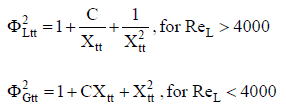
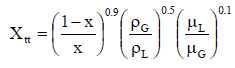
where Xtt is the Martinelli’s parameter defined as:
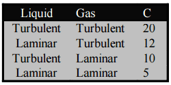 and the value of C in these equations depends on the flow regimes of the liquid and vapor. These values are in the following table.
The Lockhart-Martinelli correlation has been found to be adequate for two-phase flows at low and moderate pressures. Martinelli and Nelson’s (1948) and Thom (1964) revised models are recommended for applications at higher pressures.

Two-phase Minor Loss
Any piping system contains different technological elements in the industry, such as bends, fittings, valves, or heated channels. These additional components add to the overall head loss of the system. Such losses are generally termed minor losses, although they often account for a major portion of the head loss. For relatively short pipe systems, with a relatively large number of bends and fittings, minor losses can easily exceed major losses (especially with a partially closed valve that can cause a greater pressure loss than a long pipe when a valve is closed or nearly closed, the minor loss is infinite).
Single-phase minor losses are commonly measured experimentally. The data, especially for valves, are somewhat dependent upon the particular manufacturer’s design. The two-phase pressure loss due to local flow obstructions is treated like the single-phase frictional losses – via local loss multiplier.
See more: TWO-PHASE FRICTIONAL PRESSURE LOSS IN HORIZONTAL BUBBLY FLOW WITH 90-DEGREE BEND